This tutorial introduces the concept of Multilevel or Mixed Effects Ordinal Models and their application in analyzing hierarchical data with ordinal outcomes. Multilevel ordinal models extend the framework of linear mixed-effects models to accommodate ordinal response variables with multiple levels. This tutorial covers the following topics:
Overview
Mixed-Effects Ordinal Regression is a statistical technique used to model ordinal response variables (i.e., categorical variables with an inherent order) while accounting for both fixed effects (predictors of interest) and random effects (to capture variability due to hierarchical or grouped data structures, such as subjects, clusters, or repeated measures).
An ordinal variable \(Y\) takes values \(1, 2, \dots, K\) (where \(K\) is the number of categories), with an implicit order but unknown spacing between categories.
The ordinal outcome is often modeled using a latent continuous variable \(Y^*\):
\[ Y^* = X\beta + Zb + \epsilon\] where
\(Y^*\): Latent continuous variable.
\(X\): Fixed effects design matrix.
\(\beta\): Coefficients for fixed effects (population-level parameters).
\(Z\): Random effects design matrix.
\(b\): Random effects, typically assumed \(b \sim N(0, \Sigma_b)\).
\(\epsilon\): Error term, usually assumed \(\epsilon \sim N(0, 1)\).
The observed ordinal response \(Y\) is linked to \(Y^*\) via thresholds:
\[ Y = k \quad \text{if } \tau_{k-1} < Y^* \leq \tau_k, \quad k = 1, \dots, K \]
where \(\tau_0 = -\infty\) and \(\tau_K = \infty\), and \(\tau_1, \dots, \tau_{K-1}\) are estimated threshold parameters.
Parameters are estimated using maximum likelihood estimation (MLE) or Bayesian methods.
Multilevel Ordinal Model from Scratch
Below is a step-by-step explanation of how to fit a multilevel ordinal model from scratch in R. I’ll break it down into logical parts, matching the provided R script.
Simulate Data
We create a dataset that mimics a multilevel ordinal outcome. Here’s the logic:
Hierarchical Structure: Assume data is grouped into 20 clusters (e.g., patients nested in clinics), each with 50 observations.
Random Effects: Each group has a random intercept, drawn from a normal distribution with standard deviation \(\sigma_b = 1\).
Fixed Effect: Simulate a predictor \(x\), and let the true coefficient for \(x\)\(\beta\) be \(0.5\).
Ordinal Categories: Define thresholds that split the latent variable \(Y^*\) into ordered categories \(Y\).
Here is the simulated setup:
Code
# Step 1: Simulate Dataset.seed(123)# Define the number of groups and observations per groupn_groups <-20# Number of groups (e.g., clinics)n_obs_per_group <-50# Observations per group# True parametersbeta <-0.5# Fixed effect coefficientsigma_b <-1# Standard deviation of random interceptsthresholds <-c(-1, 0, 1) # Thresholds for ordinal categories# Simulate random intercepts for groupsgroup_random_effects <-rnorm(n_groups, mean =0, sd = sigma_b)# Simulate datadata <-data.frame(group =rep(1:n_groups, each = n_obs_per_group), # Group IDsx =rnorm(n_groups * n_obs_per_group) # Predictor variable)# Generate the latent response Y* and ordinal response Ydata$eta <- beta * data$x + group_random_effects[data$group]data$y_star <- data$eta +rnorm(nrow(data)) # Add individual noisedata$y <-cut( data$y_star,breaks =c(-Inf, thresholds, Inf),labels =1:(length(thresholds) +1),right =TRUE)data$y <-as.numeric(as.character(data$y)) # Convert factor to numerichead(data)
Fixed Effects: Use \(\beta \cdot X\) to model the population-level effect of the predictor. Random Effects: Model the group-specific random intercepts \(b_i\) using a normal distribution. Probit Link Function: Use cumulative probabilities to map latent \(Y^*\) into ordinal categories defined by thresholds.
The cumulative probabilities for each category \(k\) are:
\[ P(Y = k \mid X, b) =
\begin{cases}
\Phi(\tau_k - \eta), & k = 1 \\
\Phi(\tau_k - \eta) - \Phi(\tau_{k-1} - \eta), & 2 \leq k \leq K - 1 \\
1 - \Phi(\tau_{k-1} - \eta), & k = K
\end{cases} \]
The function computes: - Log-likelihood for observed data \(Y\), given parameters (\(\beta, \tau, b, \sigma_b\)). - Random effects prior, to incorporate their distribution.
In this section we will fit a mixed-effects ordinal regression model to the simulated data using the clmm() function from the {ordinal} package. The clmm() function fits cumulative link mixed models (CLMMs) to ordinal response data. Fits cumulative link mixed models, i.e. cumulative link models with random effects via the Laplace approximation or the standard and the adaptive Gauss-Hermite quadrature approximation. Laplace approximation is the default method for fitting the model which plays a critical role in estimating the likelihood of the model by simplifying the integration over random effects. Mixed-effects models involve random effects to account for group-level variation, but these random effects introduce high-dimensional integrals into the likelihood function, making it computationally intractable to solve exactly. The Gauss-Hermite quadrature approximation is a numerical integration technique Gauss-Hermite quadrature is particularly well-suited for integrating over Gaussian random effect which is particularly useful for computing integrals involving a Gaussian density function, as it efficiently approximates the integral by using a weighted sum of function evaluations at specific points (nodes).
Install Required R Packages
Following R packages are required to run this notebook. If any of these packages are not installed, you can install them using the code below:
The soup data from {ordinal} package has 1847 rows and 13 variables. 185 respondents participated in an A-not A discrimination test with sureness. Before experimentation the respondents were familiarized with the reference product and during experimentation, the respondents were asked to rate samples on an ordered scale with six categories given by combinations of (reference, not reference) and (sure, not sure, guess) from ‘referene, sure’ = 1 to ‘not reference, sure’ = 6. The data set contains the following variables:
RESP: factor with 185 levels: the respondents in the study.
PROD: factor with 2 levels: index reference and test products.
PRODID: factor with 6 levels: index reference and the five test product variants.
SURENESS: ordered factor with 6 levels: the respondents ratings of soup samples.
DAY:` factor with two levels: experimentation was split over two days.
SOUPTYPE: factor with three levels: the type of soup regularly consumed by the respondent.
SOUPFREQ: factor with 3 levels: the frequency with which the respondent consumes soup.
COLD: factor with two levels: does the respondent have a cold?
EASY: factor with ten levels: How easy did the respondent find the discrimation test? 1 = difficult, 10 = easy.
GENDER: factor with two levels: gender of the respondent.
AGEGROUP: factor with four levels: the age of the respondent.
LOCATION: factor with three levels: three different locations where experimentation took place.
Code
data(soup, lib ="ordinal")
Warning in data(soup, lib = "ordinal"): data set 'ordinal' not found
We fit a mixed-effects ordinal regression model to the soup data using the clmm() function from the ordinal package. The clmm() function fits cumulative link mixed models (CLMMs) to ordinal response data. CLMMs are an extension of generalized linear mixed models (GLMMs) to ordinal response data. The clmm() function allows you to specify both fixed and random effects in the model formula. The link argument specifies the link function to use, and the threshold argument specifies the type of threshold parameterization to use. The Hess argument specifies whether to compute the Hessian matrix for the model.
Ordinal Regression Model with Random Intercept
First we fit a cumulative link model with one random term (random intercept) to the soup data. The model predicts the SURENESS of soup samples based on the RESP variable (respondent ID) as a random effect. We use the link = "probit" argument to specify the probit link function and the threshold = "equidistant" argument to specify equidistant thresholds. We set Hess = TRUE to compute the Hessian matrix for the model.
Code
## Cumulative link model with one random term: m_01 <-clmm(SURENESS ~(1|RESP), link ="probit", threshold ="equidistant",Hess =TRUE,data = mf) summary(m_01)
Cumulative Link Mixed Model fitted with the Laplace approximation

formula: SURENESS ~ (1 | RESP)
data:    mf

 link   threshold   nobs logLik   AIC     niter    max.grad cond.H
 probit equidistant 1847 -2860.32 5726.63 115(319) 3.16e-05 3.8e+02

Random effects:
 Groups Name        Variance Std.Dev.
 RESP   (Intercept) 0.08037  0.2835
Number of groups:  RESP 185

No Coefficients

Threshold coefficients:
             Estimate Std. Error z value
threshold.1 -1.128753   0.041359  -27.29
spacing      0.301646   0.009349   32.27
Ordinal Regression Model with Random Intercept and Fixed Effects
Then, we fit a cumulative link model with one random term (random intercept) and fixed effects to the soup data. The model predicts the SURENESS of soup samples based on the PROD and GENDER variables as fixed effects and the RESP variable (respondent ID) as a random effect. We use the link = "probit" argument to specify the probit link function and the threshold = "equidistant" argument to specify equidistant thresholds. We set Hess = TRUE to compute the Hessian matrix for the model.
Code
## Cumulative link model with one random term and fixed effects: m_02 <-clmm(SURENESS ~ PROD + GENDER + (1|RESP),link ="probit", threshold ="equidistant",Hess =TRUE, data = mf) summary(m_02)
Cumulative Link Mixed Model fitted with the Laplace approximation

formula: SURENESS ~ PROD + GENDER + (1 | RESP)
data:    mf

 link   threshold   nobs logLik   AIC     niter    max.grad cond.H
 probit equidistant 1847 -2772.33 5554.66 245(770) 2.44e-03 2.6e+02

Random effects:
 Groups Name        Variance Std.Dev.
 RESP   (Intercept) 0.1079   0.3285
Number of groups:  RESP 185

Coefficients:
             Estimate Std. Error z value Pr(>|z|)
PRODTest      0.71193    0.05392  13.204   <2e-16 ***
GENDERFemale -0.04028    0.07609  -0.529    0.597
---
Signif. codes:  0 '***' 0.001 '**' 0.01 '*' 0.05 '.' 0.1 ' ' 1

Threshold coefficients:
            Estimate Std. Error z value
threshold.1 -0.80991    0.07219  -11.22
spacing      0.32282    0.00995   32.44
Ordinal Regression Model with Two Random Terms and Fixed Effects
Lastly, we fit a cumulative link model with two random terms (random intercept and random slope) and fixed effects to the soup data. The model predicts the SURENESS of soup samples based on the PROD and GENDER variables as fixed effects and the RESP variable (respondent ID) and the interaction between RESP and PROD as random effects. We use the link = "probit" argument to specify the probit link function and the threshold = "equidistant" argument to specify equidistant thresholds.
Code
# Cumulative link model with two random term and fixed effects: m_03 <-clmm(SURENESS ~ PROD + GENDER+(1|RESP) + (1|RESP:PROD), data = soup,link ="probit", threshold ="equidistant")summary(m_03)
Cumulative Link Mixed Model fitted with the Laplace approximation

formula: SURENESS ~ PROD + GENDER + (1 | RESP) + (1 | RESP:PROD)
data:    soup

 link   threshold   nobs logLik   AIC     niter     max.grad cond.H
 probit equidistant 1847 -2763.32 5538.63 557(1703) 1.67e-03 1.6e+02

Random effects:
 Groups    Name        Variance Std.Dev.
 RESP:PROD (Intercept) 0.14832  0.3851
 RESP      (Intercept) 0.04454  0.2110
Number of groups:  RESP:PROD 370,  RESP 185

Coefficients:
             Estimate Std. Error z value Pr(>|z|)
PRODTest      0.74209    0.06803  10.909   <2e-16 ***
GENDERFemale -0.04252    0.07830  -0.543    0.587
---
Signif. codes:  0 '***' 0.001 '**' 0.01 '*' 0.05 '.' 0.1 ' ' 1

Threshold coefficients:
            Estimate Std. Error z value
threshold.1 -0.83962    0.07693  -10.91
spacing      0.33446    0.01058   31.62
Model Comparision
We can compare the models using the anova() function to test the overall model fit. The anova() function compares the models using the likelihood ratio test, which tests whether the model with predictors is significantly better than the model without predictors.
From the above output, model with two random terms and fixed effects (m_03) is significantly better than the model with one random term and fixed effects (m_02) (p < 0.05). The model with one random term (m_02) is also significantly better than the model with no random terms (m_01) (p < 0.05).
Odds Ratio
The coefficients in the model can be hard to understand because they are scaled in logs. Another way to interpret logistic regression models is to change the coefficients into odds ratios. The odds ratio is the ratio of the odds of the event happening in one group to the odds of the event happening in another group. The odds ratio is calculated by exponentiating the coefficient.
The tab_model() function of {sjPlot} package also creates HTML tables of the model coefficients and odds ratios, CI and cxorresponding p-values.
Code
tab_model(m_03)
SURENESS
Predictors
Odds Ratios
CI
p
threshold 1
0.43
0.37 – 0.50
<0.001
spacing
1.40
1.37 – 1.43
<0.001
PROD [Test]
2.10
1.84 – 2.40
<0.001
GENDER [Female]
0.96
0.82 – 1.12
0.587
Random Effects
σ2
1.00
τ00RESP:PROD
0.15
τ00RESP
0.04
ICC
0.16
N RESP
185
N PROD
2
Observations
1847
Marginal R2 / Conditional R2
0.100 / 0.246
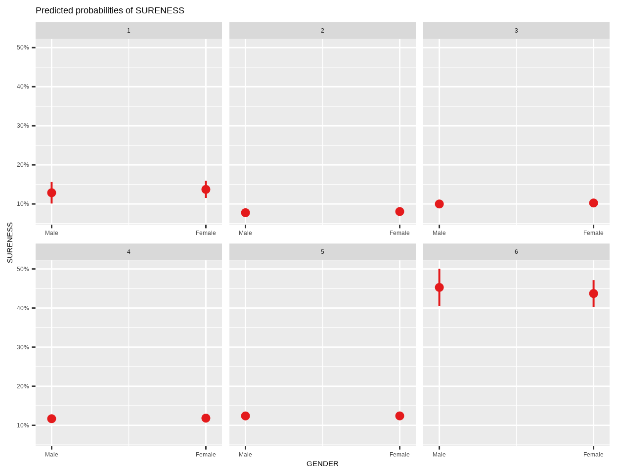
plot_model() function of {sjPlot} package creates plots the estimates from the fitted model:
Code
plot_model(m_03, type ="pred", terms =c("GENDER"))
Model Performance
We can evaluate the performance of the mixed-effects multinomial model using the performance() function from the {performance} package. This function provides various performance metrics such as the AIC, BIC, and log-likelihood of the model.
Code
performance::performance(m_03)
Can't calculate log-loss.
Can't calculate proper scoring rules for ordinal, multinomial or
  cumulative link models.
# Indices of model performance

AIC      |      BIC | R2 (cond.) | R2 (marg.) |  RMSE | Sigma
-------------------------------------------------------------
5538.631 | 5571.759 |      0.246 |      0.100 | 4.403 | 4.410
Summary and Conclusion
Mixed-effects ordinal regression models are an enhanced version of ordinal regression that accommodates hierarchical or grouped data structures. These models are particularly beneficial when the response variable is ordinal (i.e., consists of ordered categories) and when the data include random effects, such as measurements taken from multiple individuals or groups. The cumulative link mixed model (CLMM), which can be implemented using the clmm() function from the {ordinal} package in R, allows for the modeling of ordinal data with both fixed and random effects. This tutorial is a foundation for applying mixed-effects ordinal regression in real-world scenarios, enabling researchers to draw meaningful conclusions from hierarchical ordinal data.