4. Multivariate Analysis of Variance (MANOVA)

This tutorial covers the concept of Multivariate Analysis of Variance (MANOVA), a statistical technique used to analyze the differences among groups on multiple dependent variables simultaneously. MANOVA is an extension of Analysis of Variance (ANOVA) to situations where there are multiple dependent variables. It is particularly useful when the dependent variables are correlated and when researchers want to test whether the mean vectors of the dependent variables are equal across groups defined by one or more independent variables.

Overview

Multivariate Analysis of Variance (MANOVA) is a statistical method that extends Analysis of Variance (ANOVA) to situations where there are multiple dependent variables. It tests whether the mean vectors of the dependent variables are equal across groups defined by one or more independent variables. MANOVA is particularly useful when the dependent variables are correlated. MANOVA allows researchers to determine whether there are significant differences among groups on multiple dependent variables simultaneously. This can be useful when studying complex phenomena where multiple variables may be involved in explaining the outcome of interest.

MANOVA analyzes the differences among groups in an independent variable by considering multiple dependent variables. This reduces the type I error which can be inflated by performing separate univariate ANOVA for each dependent variable. MANOVA also controls for inter-correlations among the multiple dependent variables in the dataset. As compared to univariate ANOVA, MANOVA uses more information from the dependent variables i.e., MANOVA may find differences between groups based on combined information from the multiple dependent variables.

MANOVA is based on the general linear model (GLM) framework and involves estimating a set of linear equations that relate the dependent variables to the independent variables. The technique produces a set of output statistics, including F-values and p-values, that indicate whether there are significant differences among groups on the dependent variables. In contrast to ANOVA, where we compare individual group means, MANOVA compares the vectors containing the group mean of each dependent variable. MANOVA uses omnibus Wilk’s Lambda, Pillai’s Trace (most robust to departures from assumptions), Roy’s Largest Root, or Hotelling-Lawley’s test, which are later converted to F statistics for assessing the significance of the group differences. Pillai’s Trace has the highest statistical power. MANOVA maximizes the discrimination in between-groups than within-groups based on best linear combinations of the multiple response variables.

Key Concepts

  • Dependent Variables (\(Y_1, Y_2, \ldots, Y_p\)): These are the multiple outcome variables being analyzed.
  • **Dependent Variables (\(Y_1, Y_2, \ldots, Y_p\)): These are the multiple outcome variables being analyzed.
  • Independent Variable(s): These define the groups or categories being compared.
  • Hypothesis Testing: MANOVA tests the null hypothesis (\(H_0\)) that the mean vectors of the dependent variables are the same across groups.

Mathematical Formulation

Suppose there are \(k\) groups, \(p\) dependent variables, and \(n_i\) observations in the \(i\)-th group (\(n = \sum_{i=1}^k n_i\)).

1. Mean Vector

For the \(i\)-th group, the sample mean vector of the dependent variables is:

\[ \bar{\mathbf{Y}}_i = \frac{1}{n_i} \sum_{j=1}^{n_i} \mathbf{Y}_{ij} \] where \(\mathbf{Y}_{ij} = [Y_{ij1}, Y_{ij2}, \ldots, Y_{ijp}]^\top\) is the vector of dependent variable values for the \(j\)-th observation in the \(i\)-th group.

The overall mean vector is:

\[ \bar{\mathbf{Y}} = \frac{1}{n} \sum_{i=1}^k \sum_{j=1}^{n_i} \mathbf{Y}_{ij} \] 2. Hypotheses

  • Null Hypothesis (\(H_0\)): The mean vectors are equal across groups:

    \[ H_0: \bar{\mathbf{Y}}_1 = \bar{\mathbf{Y}}_2 = \cdots = \bar{\mathbf{Y}}_k \]

  • Alternative Hypothesis (\(H_A\)): At least one group mean vector differs.

3. Partitioning Variance

MANOVA partitions the total variation into:

  • Within-Group Variation (\(\mathbf{W}\)): Variation within each group.

\[ \mathbf{W} = \sum_{i=1}^k \sum_{j=1}^{n_i} (\mathbf{Y}_{ij} - \bar{\mathbf{Y}}_i)(\mathbf{Y}_{ij} - \bar{\mathbf{Y}}_i)^\top \]

  • Between-Group Variation (\(\mathbf{B}\)): Variation between group means.

\[ \mathbf{B} = \sum_{i=1}^k n_i (\bar{\mathbf{Y}}_i - \bar{\mathbf{Y}})(\bar{\mathbf{Y}}_i - \bar{\mathbf{Y}})^\top \]

The total variation is:

\[ \mathbf{T} = \mathbf{W} + \mathbf{B} \]

4. Test Statistic

Several test statistics are used in MANOVA, including:

  1. Wilks’ Lambda (\(\Lambda\)):

\[ \Lambda = \frac{\det(\mathbf{W})}{\det(\mathbf{W} + \mathbf{B})} \] Smaller values of \(\Lambda\) indicate stronger evidence against \(H_0\).

  1. Pillai’s Trace:

\[ V = \text{trace}[(\mathbf{B})(\mathbf{W} + \mathbf{B})^{-1}] \]

Larger values indicate stronger evidence against \(H_0\).

Hotelling-Lawley Trace and Roy’s Largest Root are other options.

Interpretation

If the null hypothesis is rejected, it means that the groups differ significantly in terms of their mean vectors. Follow-up analyses, such as discriminant analysis or individual ANOVAs, are often performed to explore the specific differences.

Example

Consider an experiment comparing three groups (\(k = 3\)) on two dependent variables (\(p = 2\)), such as height and weight. MANOVA would test whether the mean vectors \([\text{Height}, \text{Weight}]\) are the same for all three groups.

Assumption of MANOVA

The assumptions of Multivariate Analysis of Variance (MANOVA) are critical to ensure the validity of the results. Here are the key assumptions:

1. Multivariate Normality

  • What it means: Each group of the independent variable should follow a multivariate normal distribution for the dependent variables.
  • Implications: The joint distribution of the dependent variables within each group is normally distributed. Univariate normality for each dependent variable is necessary but not sufficient.
  • Testing: This can be assessed using tests like Mardia’s test or graphical methods such as Q-Q plots for multivariate data.

2. Homogeneity of Covariance Matrices

  • What it means: The covariance matrices of the dependent variables should be equal across all groups.
  • Why it’s important: Unequal covariance matrices may affect the test statistics (e.g., Wilks’ Lambda) used in MANOVA.
  • Testing: Box’s M test is commonly used to check this assumption. However, it is sensitive to deviations from multivariate normality.
  • Remedy if violated: Use a more robust MANOVA test, such as Pillai’s Trace, which is less sensitive to violations of this assumption.

3. Independence of Observations

  • What it means: The observations within and between groups must be independent of each other.
  • Why it’s important: Non-independence (e.g., repeated measures data) can lead to incorrect results and requires specialized methods (e.g., repeated-measures MANOVA).
  • How to ensure: Ensure proper random sampling and experimental design.

4. Absence of Multicollinearity

  • What it means: The dependent variables should not be highly correlated with each other (multicollinearity).
  • Why it’s important: High correlations between dependent variables can inflate test statistics and make the analysis unstable.
  • How to check: Examine the correlation matrix of the dependent variables. Correlations above 0.9 may indicate multicollinearity.

5. Balanced Sample Sizes (Optional but Recommended)

  • What it means: The number of observations should be approximately equal across groups.
  • Why it’s important: Unequal sample sizes can affect the robustness of test statistics, especially if homogeneity of covariance is violated.
  • Remedy if violated: Use Type III sums of squares or robust methods.

6. Linearity

  • What it means: The relationships between the dependent variables and the independent variable(s) should be linear.
  • Why it’s important: Nonlinear relationships can distort the results of MANOVA.
  • How to check: Scatterplot matrices or other graphical methods can be used.

7. Outliers

  • What it means: MANOVA is sensitive to multivariate outliers, which can skew results.
  • How to check: Use Mahalanobis distance to identify multivariate outliers.
  • Remedy if violated: Consider removing or transforming outliers, but ensure this is justified.

Summary of Assumptions and Their Importance:

Assumption Why It Matters Common Tests
Multivariate Normality Ensures valid p-values for hypothesis testing. Mardia’s Test, Q-Q plots
Homogeneity of Covariance Affects robustness of test statistics. Box’s M test
Independence Avoids misleading conclusions. Proper experimental design
Absence of Multicollinearity Prevents inflated statistics and instability. Correlation matrix, Variance Inflation Factor (VIF)
Balanced Sample Sizes Ensures robustness of tests and reduces bias. Descriptive statistics
Linearity Keeps analysis appropriate for MANOVA methods. Scatterplots
Outliers Prevents distortion of results. Mahalanobis distance, leverage plots

Violations of these assumptions may require alternative methods, transformations, or robust versions of MANOVA to ensure accurate results.

Multivariate Analysis of Variance (MANOVA) from Scratch

To perform a Multivariate Analysis of Variance (MANOVA) from scratch in R without using any packages, you would compute the necessary matrices and test statistics manually. Below is a step-by-step guide:

Data Preparation

Suppose we have the following dataset:

Code
# Example data
group <- rep(c("A", "B", "C"), each = 5)
y1 <- c(3, 2, 4, 3, 5, 7, 6, 8, 6, 7, 9, 10, 8, 10, 9)
y2 <- c(1, 3, 2, 4, 3, 8, 7, 6, 7, 8, 6, 5, 7, 6, 5)
data <- data.frame(group, y1, y2)
head(data)
  group y1 y2
1     A  3  1
2     A  2  3
3     A  4  2
4     A  3  4
5     A  5  3
6     B  7  8

Compute Group Means and Overall Mean

Compute the overall mean vector and group means:

Code
# Overall mean vector
overall_mean <- colMeans(data[, 2:3])

# Group means
group_means <- aggregate(. ~ group, data = data, FUN = mean)
group_means <- group_means[, -1]  # Remove group column

Compute \(\mathbf{H}\) and \(\mathbf{E}\)

The between-group sum of squares and within-group sum of squares matrices are computed as follows:

Code
# Initialize matrices
H <- matrix(0, ncol = 2, nrow = 2)
E <- matrix(0, ncol = 2, nrow = 2)

# Compute H (between-group)
n_groups <- table(data$group)
for (i in 1:nrow(group_means)) {
  diff <- as.matrix(group_means[i, ] - overall_mean)
  H <- H + n_groups[i] * (t(diff) %*% diff)
}

for (i in unique(data$group)) {
  group_data <- data[data$group == i, 2:3]  # Data for group i
  group_mean <- as.numeric(group_means[which(unique(data$group) == i), ])  # Group mean
  diff <- as.matrix(group_data - matrix(group_mean, nrow = nrow(group_data), ncol = ncol(group_data), byrow = TRUE))
  E <- E + t(diff) %*% diff
}

Compute Wilks’ Lambda

Compute Wilks’ Lambda, which is a measure of the proportion of variance in the dependent variables that is not explained by the independent variable:

Code
# Compute Wilks' Lambda
lambda <- det(E) / det(H + E)
lambda
[1] 0.02723586

Approximate F-statistic

Compute the F-statistic to test the significance of the group differences:

Code
# Dimensions
p <- ncol(data[, 2:3])  # Number of dependent variables
k <- length(unique(data$group))  # Number of groups
n <- nrow(data)  # Total sample size

# F-approximation
df1 <- p * (k - 1)
df2 <- n - k - p + 1
f_stat <- ((1 - lambda^(1 / p)) / lambda^(1 / p)) * (df2 / df1)
f_stat
[1] 13.91334

Determine Significance

Determine the significance of the F-statistic using the F-distribution:

Code
# P-value
p_value <- pf(f_stat, df1, df2, lower.tail = FALSE)
p_value
[1] 0.0002781186

Results Interpretation

  • \(\Lambda\): Smaller values indicate group differences.
  • \(F\)-statistic: Compare to critical value.
  • \(p\)-value: If (\(p < \alpha\)) (e.g., \(0.05\)), reject \(H_0\) and conclude significant differences among groups.

Multivariate Analysis of Variance (MANOVA) in R

Here is a list of R packages commonly used for Multivariate Analysis of Variance (MANOVA), along with a brief description of their purpose and functionality:

1. stats

  • Description: The base R package for statistical analysis.

  • Function: manova()

  • Purpose: Performs MANOVA and provides standard summary statistics for test statistics like Wilks’ Lambda, Pillai’s Trace, and Hotelling-Lawley Trace.

  • Usage:

    fit <- manova(cbind(y1, y2) ~ group, data = data)
    summary(fit, test = "Wilks")

2. car (Companion to Applied Regression)

  • Description: Provides tools for regression diagnostics and hypothesis testing.

  • Function: Manova()

  • Purpose: Enhances manova() from stats and integrates better diagnostic tools.

  • Usage:

    fit <- lm(cbind(y1, y2) ~ group, data = data)
    Manova(fit, test.statistic = "Wilks")

3. heplots - Description: Specializes in hypothesis-error (HE) plots for multivariate linear models. - Function: heplot() and Anova() - Purpose: Performs MANOVA and visualizes the relationships between hypotheses and errors using HE plots. - Usage: r fit <- lm(cbind(y1, y2) ~ group, data = data) Anova(fit) heplot(fit)

4. MASS - Description: Functions and datasets to support Modern Applied Statistics with S. - Function: manova() - Purpose: Extends statistical techniques, including MANOVA, with support for custom tests. - Usage: r fit <- manova(cbind(y1, y2) ~ group, data = data) summary(fit, test = "Pillai")

5. MANOVA.RM

  • Description: Provides functions for Robust MANOVA

  • Function: MANOVA.wide()

  • Purpose: Performs MANOVA and provides robust estimates of the group differences.

  • Usage:

    fit <- MANOVA.wide(cbind(y1, y2) ~ group, data = data)
    summary(fit)

Install Required R Packages

Following R packages are required to run this notebook. If any of these packages are not installed, you can install them using the code below:

Code
packages <- c('tidyverse', 
              'plyr',
              'flextable',
              'patchwork',
              'rstatix',
              'effectsize',
              'GGally',
              'MASS',
              'MANOVA.RM',
              'car',
              'heplots',
              'jmv'
         )
#| warning: false
#| error: false

# Install missing packages
new_packages <- packages[!(packages %in% installed.packages()[,"Package"])]
if(length(new_packages)) install.packages(new_packages)
 devtools::install_github("ItziarI/WeDiBaDis")

# Verify installation
cat("Installed packages:\n")
print(sapply(packages, requireNamespace, quietly = TRUE))

Load Packages

Code
# Load packages with suppressed messages
invisible(lapply(packages, function(pkg) {
  suppressPackageStartupMessages(library(pkg, character.only = TRUE))
}))
library(WeDiBaDis)
Code
# Check loaded packages
cat("Successfully loaded packages:\n")
Successfully loaded packages:
Code
print(search()[grepl("package:", search())])
 [1] "package:WeDiBaDis"  "package:jmv"        "package:heplots"   
 [4] "package:broom"      "package:car"        "package:carData"   
 [7] "package:MANOVA.RM"  "package:MASS"       "package:GGally"    
[10] "package:effectsize" "package:rstatix"    "package:patchwork" 
[13] "package:flextable"  "package:plyr"       "package:lubridate" 
[16] "package:forcats"    "package:stringr"    "package:dplyr"     
[19] "package:purrr"      "package:readr"      "package:tidyr"     
[22] "package:tibble"     "package:ggplot2"    "package:tidyverse" 
[25] "package:stats"      "package:graphics"   "package:grDevices" 
[28] "package:utils"      "package:datasets"   "package:methods"   
[31] "package:base"      

Data

Suppose we have a data set of different landuse (NLCD) and with SOC and NDVI, We want to see if SOC and NDVI are associated with different NLCD using MANOVA.

gp_soil_data.csv

Code
# load data
mf<-readr::read_csv("https://github.com/zia207/r-colab/raw/main/Data/Regression_analysis/gp_soil_data.csv")
glimpse(mf)
Rows: 467
Columns: 19
$ ID        <dbl> 1, 2, 3, 4, 5, 6, 7, 8, 9, 10, 11, 12, 13, 14, 15, 16, 17, 1…
$ FIPS      <dbl> 56041, 56023, 56039, 56039, 56029, 56039, 56039, 56039, 5603…
$ STATE_ID  <dbl> 56, 56, 56, 56, 56, 56, 56, 56, 56, 56, 56, 56, 56, 56, 56, …
$ STATE     <chr> "Wyoming", "Wyoming", "Wyoming", "Wyoming", "Wyoming", "Wyom…
$ COUNTY    <chr> "Uinta County", "Lincoln County", "Teton County", "Teton Cou…
$ Longitude <dbl> -111.0119, -110.9830, -110.8065, -110.7344, -110.7308, -110.…
$ Latitude  <dbl> 41.05630, 42.88350, 44.53497, 44.43289, 44.80635, 44.09124, …
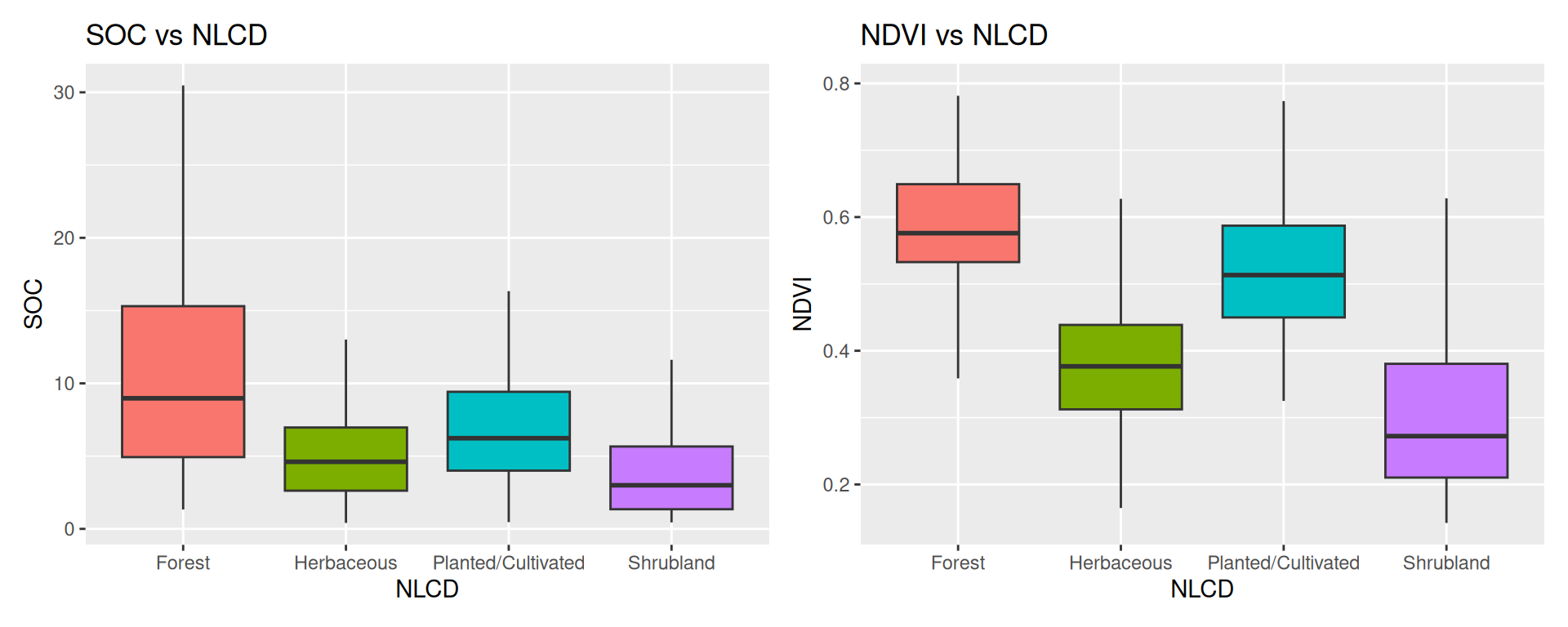
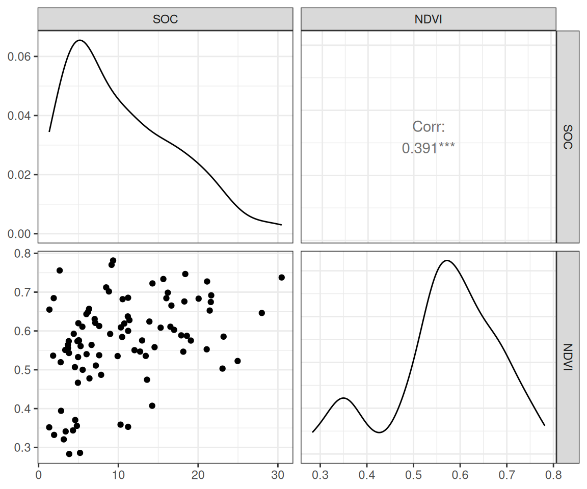
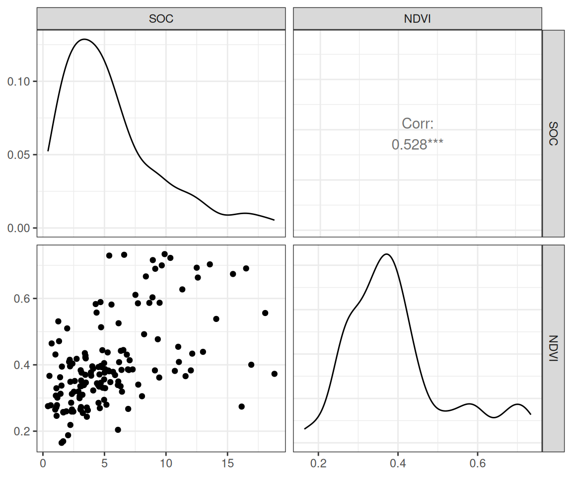
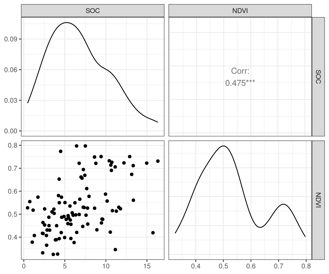
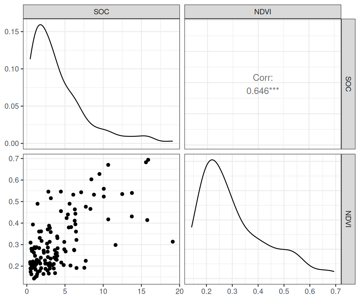
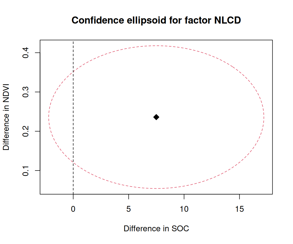
$ SOC       <dbl> 15.763, 15.883, 18.142, 10.745, 10.479, 16.987, 24.954, 6.28…
$ DEM       <dbl> 2229.079, 1889.400, 2423.048, 2484.283, 2396.195, 2360.573, …
$ Aspect    <dbl> 159.1877, 156.8786, 168.6124, 198.3536, 201.3215, 208.9732, …
$ Slope     <dbl> 5.6716146, 8.9138117, 4.7748051, 7.1218114, 7.9498644, 9.663…
$ TPI       <dbl> -0.08572358, 4.55913162, 2.60588670, 5.14693117, 3.75570583,…
$ KFactor   <dbl> 0.31999999, 0.26121211, 0.21619999, 0.18166667, 0.12551020, …
$ MAP       <dbl> 468.3245, 536.3522, 859.5509, 869.4724, 802.9743, 1121.2744,…
$ MAT       <dbl> 4.5951686, 3.8599243, 0.8855000, 0.4707811, 0.7588266, 1.358…
$ NDVI      <dbl> 0.4139390, 0.6939532, 0.5466033, 0.6191013, 0.5844722, 0.602…
$ SiltClay  <dbl> 64.84270, 72.00455, 57.18700, 54.99166, 51.22857, 45.02000, …
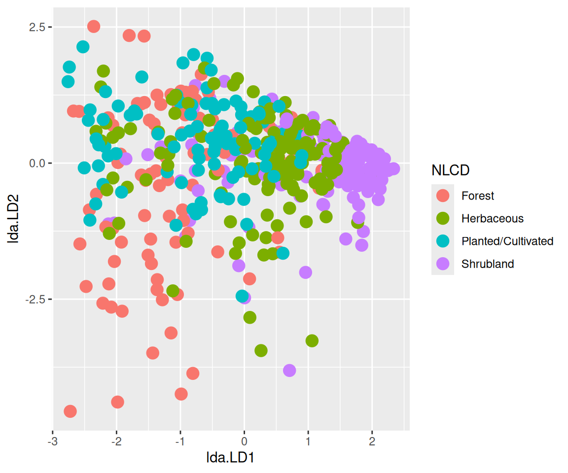
$ NLCD      <chr> "Shrubland", "Shrubland", "Forest", "Forest", "Forest", "For…
$ FRG       <chr> "Fire Regime Group IV", "Fire Regime Group IV", "Fire Regime…

Summary Statistics

Get summary statistics based on each dependent variable:

Code
# Get summary statistics of SOC
summarise_soc<-plyr::ddply(mf,~NLCD, summarise, 
                Mean= round(mean(SOC), 3),
                Median=round (median(SOC), 3),
                Min= round (min(SOC),3), 
                Max= round (max(SOC),3), 
                SD= round(sd(SOC), 3))
# Load library
library(flextable)
# Create a table
flextable::flextable(summarise_soc, theme_fun = theme_booktabs)

NLCD

Mean

Median

Min

Max

SD

Forest

10.431

8.974

1.333

30.473

6.802

Herbaceous

5.477

4.609

0.408

18.814

3.925

Planted/Cultivated

6.697

6.230

0.462

16.336

3.598

Shrubland

4.131

2.996

0.446

19.099

3.745

Code
# Get summary statistics opf NDVI
summarise_ndvi<-plyr::ddply(mf,~NLCD, summarise, 
                Mean= round(mean(NDVI), 3),
                Median=round (median(NDVI), 3),
                Min= round (min(NDVI),3), 
                Max= round (max(NDVI),3), 
                SD= round(sd(NDVI), 3))
# Load library
library(flextable)
# Create a table
flextable::flextable(summarise_ndvi, theme_fun = theme_booktabs)

NLCD

Mean

Median

Min

Max

SD

Forest

0.571

0.576

0.283

0.781

0.116

Herbaceous

0.400

0.377

0.165

0.734

0.131

Planted/Cultivated

0.533

0.513

0.325

0.797

0.121

Shrubland

0.308

0.272

0.142

0.694

0.130

Visualize the data

Code
# SOC
p1 <- ggplot(mf, aes(x = NLCD, y = SOC, fill = NLCD)) +
  geom_boxplot(outlier.shape = NA) + 
  theme(legend.position="none")+
  ggtitle("SOC vs NLCD") 

# NDVI
p2 <- ggplot(mf, aes(x = NLCD, y = NDVI, fill = NLCD)) + 
  geom_boxplot(outlier.shape = NA) + 
  theme(legend.position="none") +
  ggtitle("NDVI vs NLCD") 
Code
library(patchwork)
p1+p2

Check Assumptions of MANOVA

Before performing MANOVA, it is essential to check the assumptions of the analysis. The key assumptions of MANOVA include:

Check Normality Assumption

The Shapiro-Wilk test is used to test the normality of the dependent variables within each group. The R function shapiro_test() in the {rstatix} package can be used to perform the Shapiro-Wilk test for normality.

Code
mf %>%
  group_by(NLCD) %>%
  rstatix::shapiro_test(SOC, NDVI) %>%
  arrange(variable)
# A tibble: 8 × 4
  NLCD               variable statistic        p
  <chr>              <chr>        <dbl>    <dbl>
1 Forest             NDVI         0.948 9.51e- 4
2 Herbaceous         NDVI         0.909 4.42e- 8
3 Planted/Cultivated NDVI         0.943 3.78e- 4
4 Shrubland          NDVI         0.885 1.86e- 8
5 Forest             SOC          0.926 5.87e- 5
6 Herbaceous         SOC          0.889 3.42e- 9
7 Planted/Cultivated SOC          0.969 2.29e- 2
8 Shrubland          SOC          0.821 3.81e-11

Multivariate normality. The R function mshapiro_test() in the {rstatix} packag] can be used to perform the Shapiro-Wilk test for multivariate normality.

Code
mf   |> 
  dplyr::select(SOC, NDVI) |> 
  rstatix::mshapiro_test()
# A tibble: 1 × 2
  statistic  p.value
      <dbl>    <dbl>
1     0.856 2.77e-20

The Shapiro-Wilk test for normality shows significant results (\(p < 0.05\)) for both soil organic carbon (SOC) and the normalized difference vegetation index (NDVI), indicating that the data are not normally distributed. When the normality assumptions are unmet, you may consider transforming the outcome variables before running a MANOVA. It is also possible to conduct the MANOVA regardless, as it is generally robust to deviations from normality. However, remember that MANOVA is particularly robust when the sample size is large.

Identify multicollinearity

Compute pairwise Pearson correlation coefficients between the outcome variable. In the following R code, we’ll use the function cor_test() in {rstatix package}.

Code
mf |>  rstatix::cor_test(SOC, NDVI)
# A tibble: 1 × 8
  var1  var2    cor statistic        p conf.low conf.high method 
  <chr> <chr> <dbl>     <dbl>    <dbl>    <dbl>     <dbl> <chr>  
1 SOC   NDVI   0.59      15.6 1.35e-44    0.524     0.644 Pearson

The correlation between SOC and NDVI is 0.59, which is moderate. There is no multicollinearity between the dependent variables. In the situation, where you have multicollinearity (r >0.9), you could consider removing one of the outcome variables that is highly correlated.

Check the Homogeneity of Covariances Assumption

This can be evaluated using the Box’s M-test implemented in the rstatix package. The Box’s M-test is used to test the homogeneity of covariance matrices across groups. The null hypothesis is that the covariance matrices are equal across groups.

Code
rstatix::box_m(mf[, c("SOC", "NDVI")], mf$NLCD)
# A tibble: 1 × 4
  statistic  p.value parameter method                                           
      <dbl>    <dbl>     <dbl> <chr>                                            
1      97.3 5.61e-17         9 Box's M-test for Homogeneity of Covariance Matri…

The test results are statistically significant (p < 0.001), indicating that the assumption of homogeneity of variance-covariance matrices has been violated. If your design is balanced, meaning the groups have similar sizes, you generally do not need to be overly concerned about this violation, and you can proceed with your analysis. However, an unbalanced design can lead to issues. Possible solutions include: 1) transforming the dependent variables, or 2) continuing the analysis using Pillai’s multivariate statistic instead of Wilks statistic.

Check the Homogneity of Variance Assumption

For each of the outcome variables, the one-way MANOVA assumes that there are equal variances between groups. This can be checked using the Levene’s test of equality of variances. Key R function: levene_test() of {rstatix package}.

Code
mf |> 
  gather(key = "variable", value = "value", SOC, NDVI) |> 
  group_by(variable) %>%
  rstatix::levene_test(value ~ NLCD)
Warning: There were 2 warnings in `mutate()`.
The first warning was:
ℹ In argument: `data = map(.data$data, .f, ...)`.
Caused by warning in `leveneTest.default()`:
! group coerced to factor.
ℹ Run `dplyr::last_dplyr_warnings()` to see the 1 remaining warning.
# A tibble: 2 × 5
  variable   df1   df2 statistic        p
  <chr>    <int> <int>     <dbl>    <dbl>
1 NDVI         3   463     0.367 7.77e- 1
2 SOC          3   463    20.9   9.72e-13

The Levene’s test is significant (p < 0.05), indicating a lack of homogeneity of variances, which means this assumption has been violated. If you do not have homogeneity of variances, you can try transforming the dependent variable to address the unequal variances. Alternatively, you can proceed with your analysis, but you should accept a lower statistical significance (alpha level) level for your MANOVA results. Additionally, any follow-up univariate ANOVAs will need to be corrected for this violation, meaning you will need to use different post-hoc tests.

Check Linearity Assumption

The linearity assumption can be checked by visualizing the relationship between the dependent variables and the independent variable. A scatterplot matrix can be used to visualize the relationships between the dependent variables and the independent variable. This can be checked visually by creating a scatter plot matrix using the R function ggpairs() of {GGally} package. In our example, we have only one pair:

Code
# Create a scatterplot matrix by group
results <- mf |> 
  dplyr::select(SOC,  NDVI, NLCD) |> 
  group_by(NLCD) |> 
  rstatix::doo(~ggpairs(.) + theme_bw(), result = "plots")
results
# A tibble: 4 × 2
  NLCD               plots 
  <chr>              <list>
1 Forest             <gg>  
2 Herbaceous         <gg>  
3 Planted/Cultivated <gg>  
4 Shrubland          <gg>  
Code
results$plots
[[1]]


[[2]]


[[3]]


[[4]]

There was a linear relationship between SOC and NDVI in each NLCD as assessed by scatter plot.

Detect Multivariate Outliers

In MANOVA setting, the Mahalanobis distance is generally used to detect multivariate outliers. The distance tells us how far an observation is from the center of the cloud, taking into account the shape (covariance) of the cloud as well. The function mahalanobis_distance() in {rstatix} package can be easily used to compute the Mahalanobis distance and to flag multivariate outliers. Read more in the documentation of the function.

Code
# Compute distance by groups and filter outliers
mf |> 
dplyr::select(SOC,  NDVI, NLCD) |> 
dplyr::group_by(NLCD) |> 
rstatix:: mahalanobis_distance() |> 
filter(is.outlier == TRUE) |> 
  as.data.frame()
     SOC      NDVI mahal.dist is.outlier
1 24.954 0.5225611     17.673       TRUE
2 30.473 0.7378099     24.227       TRUE
3 19.099 0.3134793     14.077       TRUE
4 27.984 0.6462815     20.667       TRUE
5 23.058 0.5030677     14.559       TRUE

There were five multivariate outliers in the data, as assessed by Mahalanobis distance (p > 0.001). We will include the outlier in the analysis however, result will be substantially affected. This can be evaluated by comparing the result of the MANOVA with and without the outlier.

Check sample size assumption

The sample size assumption is not a strict assumption of MANOVA, but it is important to have a sufficient sample size to ensure the validity of the results. A common rule of thumb is to have at least 20 observations per group. In our example, we have 930 observations in total, with 6 groups, which meets the sample size requirement.

Code
# n in each group should be greater than number of outcome variables (SOC, NDVI)
mf |> 
  dplyr::group_by(NLCD) |> 
  dplyr::summarise(N = n())
# A tibble: 4 × 2
  NLCD                   N
  <chr>              <int>
1 Forest                93
2 Herbaceous           150
3 Planted/Cultivated    97
4 Shrubland            127

The sample size assumption is met, as each group has more than 2 outcome variables (SOC, NDVI).

Perform one-way MANOVA

In R, the manova() function of {stats} package is used to perform a Multivariate Analysis of Variance (MANOVA). The syntax for the manova function is as follows:

Code
dep_vars <- cbind(mf$SOC, mf$NDVI)
fit <- manova(dep_vars ~ NLCD, data = mf)

The output of manova() function is useful for testing whether there are significant differences between groups on multiple dependent variables. It is also useful for investigating the direction and magnitude of the effects.

Code
summary(fit)
           Df  Pillai approx F num Df den Df    Pr(>F)    
NLCD        3 0.45615   45.599      6    926 < 2.2e-16 ***
Residuals 463                                             
---
Signif. codes:  0 '***' 0.001 '**' 0.01 '*' 0.05 '.' 0.1 ' ' 1

The Pillai’s Trace test statistics is statistically significant \([Pillai's Trace = 0.4561, F(6, 926) = 45.599, p < 0.001]\) and indicates that NLCD have a statistically significant association with both combined SOC and NDVI.

Code
# get effect size
library(effectsize)
effectsize::eta_squared(fit)
# Effect Size for ANOVA (Type I)

Parameter | Eta2 (partial) |       95% CI
-----------------------------------------
NLCD      |           0.23 | [0.19, 1.00]

- One-sided CIs: upper bound fixed at [1.00].

The measure of effect size (Partial Eta Squared; ηp2) is 0.23 and suggests that there is a moderte effect of NLCD on both SOC and NDVI.

Using report() function from {report} package to get a detailed report of MANOVA:

Code
report::report(fit)
The ANOVA (formula: dep_vars ~ NLCD) suggests that:

  - The main effect of NLCD is statistically significant and large (F(3, 463) =
45.60, p < .001; Eta2 (partial) = 0.23, 95% CI [0.19, 1.00])

Effect sizes were labelled following Field's (2013) recommendations.

Post-hoc test of MANOVA

The MANOVA results suggest that there are statistically significant (p < 0.001) differences between NLCD, but it does not tell which NLCD are different from each other. To know which NLCD are significantly different, the post-hoc test needs to carry out.

To test the between-group differences, the univariate ANOVA can be done on each dependent variable, but this will be not appropriate and lose information that can be obtained from multiple variables together.

Linear discriminant analysis (LDA) is useful to show the differences between each group. LDA will discriminate the groups using information from both the dependent variables

Note

Discriminant analysis is a statistical method used to determine whether a set of variables can be used to classify observations into predefined groups. The goal of discriminant analysis is to build a predictive model that uses a set of predictor variables to classify new observations into one of several predefined groups. This can be used to understand the differences between groups, to identify the most important variables in predicting group membership, and to develop a classification rule that can be used to classify new observations.

There are two types of discriminant analysis: linear discriminant analysis (LDA) and quadratic discriminant analysis (QDA)

Discriminant analysis is commonly used for classification problems in which the classes are well-defined and the data are normally distributed. It can be used for both binary classification (i.e., separating two groups) and multi-class classification (i.e., separating more than two groups). It can also be used for feature selection, to identify the most important variables in predicting group membership.

lda() function of {MASS} package to do Linear Discriminant Analysis of group variables:

Code
library(MASS)
post_hoc <- lda(mf$NLCD ~ dep_vars, CV=F)
post_hoc
Call:
lda(mf$NLCD ~ dep_vars, CV = F)

Prior probabilities of groups:
            Forest         Herbaceous Planted/Cultivated          Shrubland 
         0.1991435          0.3211991          0.2077088          0.2719486 

Group means:
                   dep_vars1 dep_vars2
Forest             10.430882 0.5705648
Herbaceous          5.476967 0.4003461
Planted/Cultivated  6.696722 0.5332255
Shrubland           4.130764 0.3083878

Coefficients of linear discriminants:
                  LD1       LD2
dep_vars1 -0.01809082 -0.250882
dep_vars2 -7.60110166  4.955480

Proportion of trace:
   LD1    LD2 
0.9167 0.0833 

We can plot LD1 and LD2 to visualize discrimination of two predicted lda values:

Code
# create dataframe
plot_lda <- data.frame(mf[, "NLCD"], lda = predict(post_hoc)$x)
# plot
ggplot(plot_lda) + 
    geom_point(aes(x = lda.LD1, y = lda.LD2, colour =NLCD), size = 4)

The LDA scatter plot discriminates against NLCDs based on the two dependent variables. The Forest and Shurbland has a significant difference (well separated) as compared to Herbaceous and Planted/Cultivated land.

Robust MANOVA

When the assumptions of MANOVA are violated, robust versions of MANOVA can be used to provide valid results. We see that the assumptions of MANOVA are violated in our example, so we will use a robust MANOVA approach. In R, there are several approaches to robust MANOVA, including methods that account for non-normality, unequal covariance matrices, or other assumption violations. Below is an example of robust MANOVA using the {MANOVA.RM} package.

When to Use Robust MANOVA

Robust MANOVA methods are recommended when:

  • Multivariate normality is violated.

  • Covariance matrices are not homogeneous.

  • Outliers are present.

  • Sample sizes are unequal across groups.

Fit Robust MANOVA

The MANOVA.wide() function is used for data provided in wide format, i.e., with one row per unit. The formula now consists of the matrix of outcome variables (bound together via cbind()) on the left hand side of the ~ operator and the factors of interest on the right. The resampling argument specifies the type of resampling to be used: The resampling method to be used: one of paramBS (parametric bootstrap approach) and WildBS (wild bootstrap approach with Rademacher weights). The alpha argument specifies the significance level. The iter argument specifies the number of iterations for the bootstrap resampling method.

Code
fit.robust<-  MANOVA.wide(cbind(SOC, NDVI) ~ NLCD, data = mf, resampling = "paramBS",
                    alpha = 0.05, iter = 10)
summary(fit.robust)
Call: 
cbind(SOC, NDVI) ~ NLCD

Descriptive:
                NLCD   n    SOC  NDVI
1             Forest  93 10.431 0.571
2         Herbaceous 150  5.477 0.400
3 Planted/Cultivated  97  6.697 0.533
4          Shrubland 127  4.131 0.308

Wald-Type Statistic (WTS):
     Test statistic df  p-value 
NLCD "330.552"      "6" "<0.001"

modified ANOVA-Type Statistic (MATS):
     Test statistic
NLCD        392.921

p-values resampling:
     paramBS (WTS) paramBS (MATS)
NLCD "<0.001"      "<0.001"      

The robust MANOVA results show that the NLCD has a significant effect on both SOC and NDVI, even when the assumptions of MANOVA are violated. The robust MANOVA approach provides valid results even when the data do not meet the assumptions of the analysis.

Confidence Regions

Confidence regions can be calculated using the conf.reg() function. Note that confidence regions can only be plotted in designs with 2 dimensions. The conf.reg() function takes as arguments:

  • object: A MANOVA object calculated via MANOVA() or MANOVA.wide().
  • nullhypo: In designs involving more than one factor, it is necessary to specify the null hypothesis, i.e., the contrast of interest.
Code
cr <- conf.reg(fit.robust)
cr
Center: 
      [,1]
[1,] 7.494
[2,] 0.236

Scale:
[1] 3.96659975 0.07427353

Eigenvectors:
     [,1] [,2]
[1,]   -1    0
[2,]    0   -1

plot() function can be used to visualize the confidence regions:

Code
plot(cr, col = 2, lty = 2, xlab = "Difference in SOC", ylab ="Difference in NDVI")

The output includes the essential parameters for defining the ellipsoid: the center, the eigenvectors that determine the axes of the ellipsoid, and the scaling factors for these eigenvectors. The scaling factors are derived from the eigenvalues, the bootstrap quantile, and the total sample size.

Post-hoc comparisons

We can perform post-hoc pairwise comparisons using Tukey contrasts to determine which groups differ significantly from each other. The simCI() function is used to calculate the confidence intervals for the pairwise comparisons. The contrast argument specifies the type of contrast to be used (e.g., pairwise). The type argument specifies the type of contrast to be used (e.g., Tukey).

Code
# pairwise comparison using Tukey contrasts
simCI(fit.robust, contrast = "pairwise", type = "Tukey")

 #------ Call -----# 
 
 - Contrast:  Tukey 
 - Confidence level: 95 % 

 #------Multivariate post-hoc comparisons: p-values -----# 
 
                         contrast p.value
1             Herbaceous - Forest     0.0
2     Planted/Cultivated - Forest     0.1
3              Shrubland - Forest     0.0
4 Planted/Cultivated - Herbaceous     0.1
5          Shrubland - Herbaceous     0.1
6  Shrubland - Planted/Cultivated     0.0

 #-----------Confidence intervals for summary effects-------------# 
 
                                Estimate      Lower      Upper
Herbaceous - Forest               -5.125 -8.3157480 -1.9342520
Planted/Cultivated - Forest       -3.772 -7.0435811 -0.5004189
Shrubland - Forest                -6.563 -9.7742338 -3.3517662
Planted/Cultivated - Herbaceous    1.353 -0.6492478  3.3552478
Shrubland - Herbaceous            -1.438 -3.3400452  0.4640452
Shrubland - Planted/Cultivated    -2.791 -4.8257349 -0.7562651

Factorial MANOVA

Factorial Multivariate Analysis of Variance (Factorial MANOVA) extends MANOVA to analyze the effects of two or more categorical independent variables (factors) on multiple dependent variables simultaneously. It also evaluates interactions between factors. Factorial MANOVA is useful when researchers want to examine the combined effects of multiple factors on a set of dependent variables.

Key Features of Factorial MANOVA include:

  1. Multiple Independent Variables (Factors):
    • Factorial MANOVA examines the effects of multiple factors (e.g., gender and treatment group) on the dependent variables.
  2. Interactions:
    • It assesses whether the effect of one factor depends on the levels of another factor.
  3. Multiple Dependent Variables:
    • It tests for differences in mean vectors across groups defined by the combinations of factor levels.

Suppose:

  • There are \(p\) dependent variables (\(Y_1, Y_2, \dots, Y_p\)).
  • There are two independent variables (factors) \(A\) and \(B\):
    • \(A\) has \(a\) levels.
    • \(B\) has \(b\) levels.
  • The observations are denoted by \(\mathbf{Y}_{ijk}\), where \(i\) refers to the level of \(A\), \(j\) refers to the level of $(B, and \(k\) indexes observations within each combination of \(A\) and \(B\).

For each combination of \(A\) and \(B\), the mean vector is:

\[ \bar{\mathbf{Y}}_{ij} = \frac{1}{n_{ij}} \sum_{k=1}^{n_{ij}} \mathbf{Y}_{ijk} \]

where \(n_{ij}\) is the number of observations in the \(i\)-th level of \(A\) and the \(j\)-th level of \(B\).

Fit Factorial ANOVA

First we will fit a Factorial ANOVA model with two factors, FRG and NLCD and their interaction. The lm() function is used to fit the model, and -1 removes the intercept effect

Code
# Fit a ANOVA model with interaction
fit.fact.anova <-lm(cbind(SOC, NDVI) ~ FRG + NLCD + FRG*NLCD-1, data =mf)
# Summary of results
summary(fit.fact.anova)
Response SOC :

Call:
lm(formula = SOC ~ FRG + NLCD + FRG * NLCD - 1, data = mf)

Residuals:
    Min      1Q  Median      3Q     Max 
-8.9130 -2.8293 -0.9727  2.1691 20.2000 

Coefficients: (2 not defined because of singularities)
                                                Estimate Std. Error t value
FRGFire Regime Group I                            5.2534     1.2789   4.108
FRGFire Regime Group II                           5.6658     2.6868   2.109
FRGFire Regime Group III                         10.2730     0.5767  17.812
FRGFire Regime Group IV                          13.3175     1.2789  10.414
FRGFire Regime Group V                           14.1115     1.4009  10.073
FRGIndeterminate FRG                              3.4143     3.6172   0.944
NLCDHerbaceous                                    2.6186     3.3835   0.774
NLCDPlanted/Cultivated                            2.0026     4.6110   0.434
NLCDShrubland                                    -2.6607     2.5577  -1.040
FRGFire Regime Group II:NLCDHerbaceous           -2.7584     3.9425  -0.700
FRGFire Regime Group III:NLCDHerbaceous          -7.5687     3.7365  -2.026
FRGFire Regime Group IV:NLCDHerbaceous          -14.7966     4.7851  -3.092
FRGFire Regime Group V:NLCDHerbaceous            -8.1846     4.8191  -1.698
FRGIndeterminate FRG:NLCDHerbaceous              -4.2519     5.5744  -0.763
FRGFire Regime Group II:NLCDPlanted/Cultivated   -0.9068     5.0430  -0.180
FRGFire Regime Group III:NLCDPlanted/Cultivated  -5.0496     5.6042  -0.901
FRGFire Regime Group IV:NLCDPlanted/Cultivated  -12.5601     6.5209  -1.926
FRGFire Regime Group V:NLCDPlanted/Cultivated   -12.4944     5.4558  -2.290
FRGIndeterminate FRG:NLCDPlanted/Cultivated       4.1971     6.3943   0.656
FRGFire Regime Group II:NLCDShrubland                 NA         NA      NA
FRGFire Regime Group III:NLCDShrubland           -2.8626     2.7439  -1.043
FRGFire Regime Group IV:NLCDShrubland            -5.9615     2.9182  -2.043
FRGFire Regime Group V:NLCDShrubland             -8.1158     3.8790  -2.092
FRGIndeterminate FRG:NLCDShrubland                    NA         NA      NA
                                                Pr(>|t|)    
FRGFire Regime Group I                          4.75e-05 ***
FRGFire Regime Group II                          0.03552 *  
FRGFire Regime Group III                         < 2e-16 ***
FRGFire Regime Group IV                          < 2e-16 ***
FRGFire Regime Group V                           < 2e-16 ***
FRGIndeterminate FRG                             0.34572    
NLCDHerbaceous                                   0.43939    
NLCDPlanted/Cultivated                           0.66428    
NLCDShrubland                                    0.29879    
FRGFire Regime Group II:NLCDHerbaceous           0.48451    
FRGFire Regime Group III:NLCDHerbaceous          0.04340 *  
FRGFire Regime Group IV:NLCDHerbaceous           0.00211 ** 
FRGFire Regime Group V:NLCDHerbaceous            0.09014 .  
FRGIndeterminate FRG:NLCDHerbaceous              0.44601    
FRGFire Regime Group II:NLCDPlanted/Cultivated   0.85739    
FRGFire Regime Group III:NLCDPlanted/Cultivated  0.36806    
FRGFire Regime Group IV:NLCDPlanted/Cultivated   0.05473 .  
FRGFire Regime Group V:NLCDPlanted/Cultivated    0.02248 *  
FRGIndeterminate FRG:NLCDPlanted/Cultivated      0.51192    
FRGFire Regime Group II:NLCDShrubland                 NA    
FRGFire Regime Group III:NLCDShrubland           0.29738    
FRGFire Regime Group IV:NLCDShrubland            0.04165 *  
FRGFire Regime Group V:NLCDShrubland             0.03698 *  
FRGIndeterminate FRG:NLCDShrubland                    NA    
---
Signif. codes:  0 '***' 0.001 '**' 0.01 '*' 0.05 '.' 0.1 ' ' 1

Residual standard error: 4.43 on 445 degrees of freedom
Multiple R-squared:  0.7155,    Adjusted R-squared:  0.7014 
F-statistic: 50.87 on 22 and 445 DF,  p-value: < 2.2e-16


Response NDVI :

Call:
lm(formula = NDVI ~ FRG + NLCD + FRG * NLCD - 1, data = mf)

Residuals:
     Min       1Q   Median       3Q      Max 
-0.30164 -0.08623 -0.02120  0.05673  0.36365 

Coefficients: (2 not defined because of singularities)
                                                Estimate Std. Error t value
FRGFire Regime Group I                           0.43886    0.03473  12.638
FRGFire Regime Group II                          0.39297    0.07296   5.386
FRGFire Regime Group III                         0.58753    0.01566  37.515
FRGFire Regime Group IV                          0.60858    0.03473  17.525
FRGFire Regime Group V                           0.58288    0.03804  15.322
FRGIndeterminate FRG                             0.30531    0.09822   3.108
NLCDHerbaceous                                   0.28693    0.09188   3.123
NLCDPlanted/Cultivated                           0.25545    0.12521   2.040
NLCDShrubland                                   -0.12408    0.06945  -1.786
FRGFire Regime Group II:NLCDHerbaceous          -0.27441    0.10706  -2.563
FRGFire Regime Group III:NLCDHerbaceous         -0.51752    0.10146  -5.101
FRGFire Regime Group IV:NLCDHerbaceous          -0.67175    0.12994  -5.170
FRGFire Regime Group V:NLCDHerbaceous           -0.54056    0.13086  -4.131
FRGIndeterminate FRG:NLCDHerbaceous             -0.41597    0.15137  -2.748
FRGFire Regime Group II:NLCDPlanted/Cultivated  -0.12199    0.13694  -0.891
FRGFire Regime Group III:NLCDPlanted/Cultivated -0.25002    0.15218  -1.643
FRGFire Regime Group IV:NLCDPlanted/Cultivated  -0.45680    0.17707  -2.580
FRGFire Regime Group V:NLCDPlanted/Cultivated   -0.28934    0.14815  -1.953
FRGIndeterminate FRG:NLCDPlanted/Cultivated      0.17068    0.17363   0.983
FRGFire Regime Group II:NLCDShrubland                 NA         NA      NA
FRGFire Regime Group III:NLCDShrubland          -0.14484    0.07451  -1.944
FRGFire Regime Group IV:NLCDShrubland           -0.15421    0.07924  -1.946
FRGFire Regime Group V:NLCDShrubland            -0.17602    0.10533  -1.671
FRGIndeterminate FRG:NLCDShrubland                    NA         NA      NA
                                                Pr(>|t|)    
FRGFire Regime Group I                           < 2e-16 ***
FRGFire Regime Group II                         1.17e-07 ***
FRGFire Regime Group III                         < 2e-16 ***
FRGFire Regime Group IV                          < 2e-16 ***
FRGFire Regime Group V                           < 2e-16 ***
FRGIndeterminate FRG                             0.00200 ** 
NLCDHerbaceous                                   0.00191 ** 
NLCDPlanted/Cultivated                           0.04192 *  
NLCDShrubland                                    0.07471 .  
FRGFire Regime Group II:NLCDHerbaceous           0.01070 *  
FRGFire Regime Group III:NLCDHerbaceous         5.02e-07 ***
FRGFire Regime Group IV:NLCDHerbaceous          3.55e-07 ***
FRGFire Regime Group V:NLCDHerbaceous           4.32e-05 ***
FRGIndeterminate FRG:NLCDHerbaceous              0.00624 ** 
FRGFire Regime Group II:NLCDPlanted/Cultivated   0.37349    
FRGFire Regime Group III:NLCDPlanted/Cultivated  0.10110    
FRGFire Regime Group IV:NLCDPlanted/Cultivated   0.01021 *  
FRGFire Regime Group V:NLCDPlanted/Cultivated    0.05144 .  
FRGIndeterminate FRG:NLCDPlanted/Cultivated      0.32616    
FRGFire Regime Group II:NLCDShrubland                 NA    
FRGFire Regime Group III:NLCDShrubland           0.05254 .  
FRGFire Regime Group IV:NLCDShrubland            0.05228 .  
FRGFire Regime Group V:NLCDShrubland             0.09539 .  
FRGIndeterminate FRG:NLCDShrubland                    NA    
---
Signif. codes:  0 '***' 0.001 '**' 0.01 '*' 0.05 '.' 0.1 ' ' 1

Residual standard error: 0.1203 on 445 degrees of freedom
Multiple R-squared:  0.9364,    Adjusted R-squared:  0.9333 
F-statistic:   298 on 22 and 445 DF,  p-value: < 2.2e-16

Fit Factorial MANOVA

The manova() function is used to perform a Factorial MANOVA in R. The syntax for the manova function is as follows:

Code
fit.fact.manova <-manova(cbind(SOC, NDVI) ~ FRG + NLCD + FRG*NLCD-1, data =mf)
# Summary of results
summary(fit.fact.manova)
           Df  Pillai approx F num Df den Df  Pr(>F)    
FRG         6 0.98978   72.666     12    890 < 2e-16 ***
NLCD        3 0.44076   41.931      6    890 < 2e-16 ***
FRG:NLCD   13 0.13974    2.571     26    890 3.1e-05 ***
Residuals 445                                           
---
Signif. codes:  0 '***' 0.001 '**' 0.01 '*' 0.05 '.' 0.1 ' ' 1

The results of the Factorial MANOVA show that the main effects of FRG and NLCD are significant, as well as the interaction between FRG and NLCD. This indicates that both FRG and NLCD have a significant effect on SOC and NDVI, and that the effect of FRG on SOC and NDVI depends on the level of NLCD.

Code
report::report(fit.fact.manova)
The ANOVA (formula: cbind(SOC, NDVI) ~ FRG + NLCD + FRG * NLCD - 1) suggests
that:

  - The main effect of FRG is statistically significant and large (F(6, 445) =
72.67, p < .001; Eta2 (partial) = 0.49, 95% CI [0.46, 1.00])
  - The main effect of NLCD is statistically significant and large (F(3, 445) =
41.93, p < .001; Eta2 (partial) = 0.22, 95% CI [0.18, 1.00])
  - The interaction between FRG and NLCD is statistically significant and medium
(F(13, 445) = 2.57, p < .001; Eta2 (partial) = 0.07, 95% CI [0.02, 1.00])

Effect sizes were labelled following Field's (2013) recommendations.

Multivariate Analysis of Covariance (MANCOVA)

Multivariate Analysis of Covariance (MANCOVA) is an extension of MANOVA that includes one or more continuous covariates in the analysis. MANCOVA is used to test for group differences on multiple dependent variables while controlling for the effects of one or more continuous covariates. The covariates are included as additional predictors in the model to account for their influence on the dependent variables.

The mancova() function of {jmv} is used to perform a MANCOVA in R for exploring the relationship between multiple dependent variables, and one or more categorical and/or continuous explanatory variables.

Here below is an example where we use MANCOVA to test the effects of NLCD and FRG on SOC and NDVI while controlling for the effects of MAP and MAT as covariates.

Code
fit.mancova <-mancova(data = mf,
    deps = vars(SOC, NDVI),
    factors = vars(NLCD,FRG),
    covs = vars(MAP, MAT),
    boxM = TRUE,
    multivar = list("pillai", "wilks"))
    
print(fit.mancova)

 MANCOVA

 Multivariate Tests                                                                     
 ────────────────────────────────────────────────────────────────────────────────────── 
                                 value         F             df1    df2    p            
 ────────────────────────────────────────────────────────────────────────────────────── 
   NLCD        Pillai's Trace    0.76247799     90.982287      6    886    < .0000001   
               Wilks' Lambda      0.2804653    130.869457      6    884    < .0000001   
                                                                                        
   FRG         Pillai's Trace    0.09170042      4.257538     10    886     0.0000082   
               Wilks' Lambda      0.9095108      4.293296     10    884     0.0000072   
                                                                                        
   NLCD:FRG    Pillai's Trace    0.14957347      2.754502     26    886     0.0000071   
               Wilks' Lambda      0.8518922      2.837198     26    884     0.0000036   
                                                                                        
   MAP         Pillai's Trace    0.67001534    448.728104      2    442    < .0000001   
               Wilks' Lambda      0.3299847    448.728104      2    442    < .0000001   
                                                                                        
   MAT         Pillai's Trace    0.24208298     70.588651      2    442    < .0000001   
               Wilks' Lambda      0.7579170     70.588651      2    442    < .0000001   
 ────────────────────────────────────────────────────────────────────────────────────── 


 Univariate Tests                                                                                            
 ─────────────────────────────────────────────────────────────────────────────────────────────────────────── 
                Dependent Variable    Sum of Squares    df     Mean Square       F              p            
 ─────────────────────────────────────────────────────────────────────────────────────────────────────────── 
   NLCD         SOC                     2300.2493377      3     766.749779229     51.1478639    < .0000001   
                NDVI                       4.8594674      3       1.619822453    331.2498741    < .0000001   
   FRG          SOC                      341.9780517      5      68.395610346      4.5624915     0.0004552   
                NDVI                       0.1213852      5       0.024277038      4.9645970     0.0001958   
   NLCD:FRG     SOC                       73.0094698     13       5.616113059      0.3746362     0.9772542   
                NDVI                       0.3468075     13       0.026677502      5.4554862    < .0000001   
   MAP          SOC                     1737.0904335      1    1737.090433541    115.8767404    < .0000001   
                NDVI                       4.1823672      1       4.182367204    855.2842366    < .0000001   
   MAT          SOC                      769.2951318      1     769.295131785     51.3176577    < .0000001   
                NDVI                       0.5313044      1       0.531304401    108.6504978    < .0000001   
   Residuals    SOC                     6640.9450181    443      14.990846542                                
                NDVI                       2.1662841    443       0.004890032                                
 ─────────────────────────────────────────────────────────────────────────────────────────────────────────── 


 ASSUMPTION CHECKS

 Box's Homogeneity of Covariance Matrices Test 
 ───────────────────────────────────────────── 
   χ²     df    p             
 ───────────────────────────────────────────── 
     ᵃ    63              ᵃ   
 ───────────────────────────────────────────── 
   ᵃ Too few observations to calculate
   statistic. Each (sub)group must have at
   least as many observations as there are
   dependent variables.

Summary and Conclusion

In this tutorial, we learned about Multivariate Analysis of Variance (MANOVA) and how to perform MANOVA in R. MANOVA is a powerful statistical technique that allows researchers to test for differences among groups on multiple dependent variables simultaneously. It is particularly useful when the dependent variables are correlated and when researchers want to control for inter-correlations among the dependent variables. MANOVA provides a more comprehensive analysis of group differences than univariate ANOVA and can help researchers understand the complex relationships among multiple variables. We also discussed the assumptions of MANOVA and how to check these assumptions using R. When the assumptions of MANOVA are violated, robust MANOVA methods can be used to provide valid results. We also learned about Factorial MANOVA, which extends MANOVA to analyze the effects of multiple independent variables and their interactions on multiple dependent variables. Factorial MANOVA is useful for studying the combined effects of multiple factors on a set of dependent variables. Overall, MANOVA is a versatile and powerful technique that can be used to analyze complex data sets and test hypotheses about group differences in multiple dependent variables.

References

  1. MANOVA Test in R: Multivariate Analysis of Variance

  2. MANOVA (Multivariate Analysis of Variance) using R

  3. ANOVA/MANOVA

  4. Robust MNOVA