Count data is commonly encountered in various fields, such as ecology, epidemiology, and social sciences. Poisson regression is a widely used model for analyzing this type of data, where the outcome variable represents the count of occurrences of a specific event. For instance, in epidemiology, researchers might apply Poisson regression to model the number of new disease cases that arise per unit of time within a population.
This tutorial will provide a comprehensive introduction to Poisson regression for count data in R. We will begin with an overview of the Poisson regression model and then implement it from scratch to gain a deeper understanding of its mechanics. Next, we will learn how to fit the model using R’s glm() function for practical applications. Finally, we will explore evaluation techniques, including calculating the incidence rate ratio (IRR), a crucial interpretive tool in count data models.
Overview
Poisson Regression is a type of Generalized Linear Model (GLM) used for modeling count data. Standard Poisson Regression Model considers only the number of events and does not take into account any additional exposure or observation time.
It is particularly useful when the dependent variable represents the number of occurrences of an event over a fixed period of time, space, or some other exposure, and the data exhibit a Poisson distribution. Standard Poisson Regression Model considers only the number of events and does not take into account any additional exposure or observation time.
Key characteristics of Poisson Regression:
Count Data: The response variable \(Y\) is a non-negative integer representing counts (0, 1, 2, …).
Poisson Distribution: The response variable \(Y\) follows a Poisson distribution with parameter \(\lambda\) where \(\lambda\) is the expected count. The Poisson distribution assumes that the mean and variance of the response variable are equal.
\[ Y_i \sim \text{Poisson}(\lambda_i) \]
Log Link Function: The model uses a logarithmic link function to relate the linear predictor to the Poisson mean, \(\lambda\), which ensures that the expected value \(\lambda\) is positive.
\[ \log(\lambda_i) = X_i \beta \]
Where:

-   $\lambda_i$ = $E(Y_i | X)$ is the expected count for the $i^{th}$ observation.
-   $X_i$ is the vector of predictor variables for the $i^{th}$ observation.
-   $\beta$ is the vector of coefficients to be estimated.
Model Formulation:
The Poisson regression model assumes that the log of the expected count (rate) of the dependent variable (Y) is a linear combination of the predictor variables \(X_1, X_2, \dots, X_p\). The model can be written as:
Here: - \(\lambda_i\) is the expected count (mean) of the dependent variable for the \((i^{th}\) observation. - \(\beta_0\) is the intercept. - \(\beta_1, \dots, \beta_p\) are the regression coefficients that quantify the effect of the predictor variables on the expected count.
Interpretation of Coefficients:
Intercept\(\beta_0\): The log of the expected count when all predictors are zero.
Predictor Coefficients\(\beta_1, \beta_2, \dots\): A one-unit increase in a predictor \(X_j\) is associated with a multiplicative effect on the expected count, given by \(e^{\beta_j}\). For example:
\[ e^{\beta_j} = \frac{\lambda_i(\text{new value of } X_j)}{\lambda_i(\text{old value of } X_j)} \]
This indicates the factor by which the expected count \(\lambda_i\) changes for a one-unit increase in (X_j), holding other variables constant.
Poisson Probability Mass Function (PMF):
The probability mass function of the Poisson distribution is given by:
Where \(\lambda\) is the mean count (expected value) and \(y\) is the observed count.
Interpretation of Results:
The coefficients from the model will indicate how a one-unit change in the predictor (e.g., age or income) affects the log of the expected count of accidents.
The exponentiated coefficients (exp(coef)) can be interpreted as the multiplicative change in the expected number of accidents for a one-unit increase in the predictor.
Model Assumptions:
Mean-Variance Equality: The Poisson model assumes that the mean and variance of the response variable are equal. If the data exhibit overdispersion (variance greater than the mean), the standard Poisson model may not be appropriate, and you may need to use an alternative like the Negative Binomial regression.
Independence of Observations: The counts for each observation are assumed to be independent.
Linearity on Log Scale: The log of the expected count is assumed to be a linear function of the predictor variables.
This model is widely used for count data where the occurrence of events is rare and spread over time or space, such as disease incidence, traffic accidents, or insurance claims.
Standard Poisson Regression Model
Here’s how we can fit a standard Poisson regression model manually in R using count data. Let’s assume your dataset contains a response variable y (count data) and four predictor variables \(X_1, X_2, \dots, X_4\).
Create Dataset
Code
# Set seed for reproducibilityset.seed(123)# Generate sample data with 4 predictorsn <-100x1 <-rnorm(n)x2 <-rnorm(n)x3 <-rnorm(n)x4 <-rnorm(n)# True coefficientsbeta0_true <-0.5beta1_true <-0.3beta2_true <--0.2beta3_true <-0.4beta4_true <-0.1# Calculate lambda (mean of the Poisson) for each observationlambda <-exp(beta0_true + beta1_true * x1 + beta2_true * x2 + beta3_true * x3 + beta4_true * x4)# Generate response variable y as count datay <-rpois(n, lambda)# Combine into a data framedata <-data.frame(y, x1, x2, x3, x4)head(data)
Use the optim() function to maximize the log-likelihood and obtain parameter. It is a eneral-purpose optimization based on Nelder–Mead, quasi-Newton and conjugate-gradient algorithms. It includes an option for box-constrained optimization and simulated annealing.
Code
# Initial guesses for beta0 to beta4initial_params <-c(0, 0, 0, 0, 0)# Use optim to find MLE for the parametersfit <-optim(par = initial_params, # Initial values for the parameters to be optimized over.fn = poisson_log_likelihood,hessian =TRUE) # Should a numerically differentiated Hessian matrix be returned# Extract parameter estimatesparams_hat <- fit$parcat("Estimated coefficients:", params_hat, "\n")
After fitting the Poisson regression model manually with optim(), we can calculate the standard errors, Z-scores, and P-values of the estimated coefficients. Here’s how:
Calculate the Hessian matrix: The Hessian matrix is the matrix of second derivatives of the log-likelihood function with respect to the parameters. The inverse of the Hessian provides an estimate of the variance-covariance matrix of the parameter estimates.
Extract standard errors from the variance-covariance matrix.
Calculate Z-scores and P-values based on standard errors.
Let’s implement these steps in R.
Code
# Invert the Hessian matrix to get the covariance matrixcov_matrix <-solve(fit$hessian)# Standard errorsstd_errors <-sqrt(diag(cov_matrix))# Z-scoresz_scores <- params_hat / std_errors# P-values (2-sided)p_values <-2* (1-pnorm(abs(z_scores)))# Create summary statistics tablesummary_table <-data.frame(Estimate = params_hat,Std.Error = std_errors,Z.value = z_scores,P.value = p_values)# Set row names as parameter namesrownames(summary_table) <-c("Intercept", "x1", "x2", "x3", "x4")# Display summary tableprint(summary_table)
This manual approach should yield parameter estimates that are very close to those obtained by glm(), as both methods maximize the same likelihood function.
Standard Poisson Model with R
In this exercise we will develop a standard Poisson model in R with a built function glm()to explain the variability the total diagnosed diabetes per county (count data) in the USA.
Check and Install Required R packages
Following R packages are required to run this notebook. If any of these packages are not installed, you can install them using the code below:
Physical_Inactivity: % adult access to exercise opportunities (County Health Ranking)
SVI - Level of social vulnerability in the county relative to other counties in the nation or within the state.ocial vulnerability refers to the potential negative effects on communities caused by external stresses on human health. The CDC/ATSDR Social vulnerability Index (SVI) ranks all US counties on 15 social factors, including poverty, lack of vehicle access, and crowded housing, and groups them into four related themes. ( CDC/ATSDR Social Vulnerability Index (SVI))
Food_Env_Index: Measure of access to healthy food. The Food Environment Index ranges from a scale of 0 (worst) to 10 (best) and equally weights two indicators: 1) Limited access to healthy foods based on distance an individual lives from a grocery store or supermarket, locations for healthy food purchases in most communities; and 2) Food insecurity defined as the inability to access healthy food because of cost barriers.County Health Ranking
We will use read_csv() function of {readr} package to import data as a tidy data.
Rows: 3107 Columns: 15
── Column specification ────────────────────────────────────────────────────────
Delimiter: ","
chr  (3): State, County, Urban_Rural
dbl (12): FIPS, X, Y, POP_Total, Diabetes_count, Diabetes_per, Obesity, Acce...

ℹ Use `spec()` to retrieve the full column specification for this data.
ℹ Specify the column types or set `show_col_types = FALSE` to quiet this message.
# data processingdf$Diabetes_count<-as.integer(df$Diabetes_count) df$Urban_Rural<-as.factor(df$Urban_Rural)
Data Description
The {epidisplay} package can provide both numerical and categorical statistics simultaneously with the codebook() function. It’s a great tool for descriptive statistics.
Code
epiDisplay::codebook(df[,1:7])
Diabetes_count   :

No. of observations = 3107

  Var. name      obs. mean    median  s.d.     min.   max.
1 Diabetes_count 3107 7733.95 2078    23560.52 17     703508

 ==================
Obesity      :

No. of observations = 3107

  Var. name obs. mean   median  s.d.   min.   max.
1 Obesity   3107 27.59  27.86   4.8    12.06  42.12

 ==================
Physical_Inactivity      :

No. of observations = 3107

  Var. name           obs. mean   median  s.d.   min.   max.
1 Physical_Inactivity 3107 21.16  20.84   4.3    9.64   36.72

 ==================
Access_Excercise     :

No. of observations = 3107

  Var. name        obs. mean   median  s.d.   min.   max.
1 Access_Excercise 3107 61.98  64      21.78  0      100

 ==================
Food_Env_Index   :

No. of observations = 3107

  Var. name      obs. mean   median  s.d.   min.   max.
1 Food_Env_Index 3107 7.32   7.5     1.09   1.6    10

 ==================
SVI      :

No. of observations = 3107

  Var. name obs. mean   median  s.d.   min.   max.
1 SVI       3107 0.5    0.5     0.29   0      1

 ==================
Urban_Rural      :

No. of observations = 3107

  Var. name   obs. mean   median  s.d.   min.   max.
1 Urban_Rural

 ==================
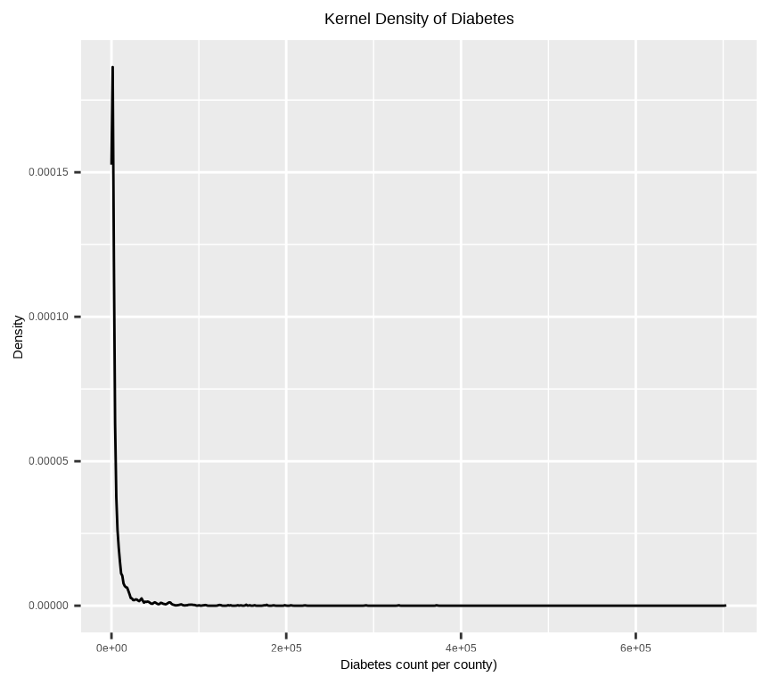
Density Plot
Code
ggplot(df, aes(Diabetes_count)) +geom_density()+# x-axis titlexlab("Diabetes count per county)") +# y-axis titleylab("Density")+# plot titleggtitle("Kernel Density of Diabetes")+theme(# Center the plot titleplot.title =element_text(hjust =0.5))
The following object is masked from 'package:jtools':

    theme_apa
The following object is masked from 'package:gtsummary':

    continuous_summary
The following object is masked from 'package:purrr':

    compose
Code
# Create a tableflextable::flextable(summarise_diabetes, theme_fun = theme_booktabs)
Urban_Rural
Mean
Median
Min
Max
SD
SE
Rural
1,169.59
875
17
7,367
1,037.88
28.676
Urban
12,519.33
4,438
24
703,508
30,080.86
709.604
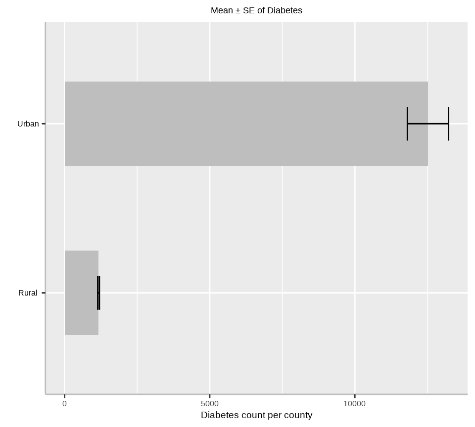
Barplot - Urban vs Rural
Code
ggplot(summarise_diabetes, aes(x=Urban_Rural, y=Mean)) +geom_bar(stat="identity", position=position_dodge(),width=0.5, fill="gray") +geom_errorbar(aes(ymin=Mean-SE, ymax=Mean+SE), width=.2,position=position_dodge(.9))+# add y-axis title and x-axis title leave blanklabs(y="Diabetes count per county", x ="")+# add plot titleggtitle("Mean ± SE of Diabetes")+coord_flip()+# customize plot themestheme(axis.line =element_line(colour ="gray"),# plot title position at centerplot.title =element_text(hjust =0.5),# axis title font sizeaxis.title.x =element_text(size =14), # X and axis font sizeaxis.text.y=element_text(size=12,vjust =0.5, hjust=0.5, colour='black'),axis.text.x =element_text(size=12))
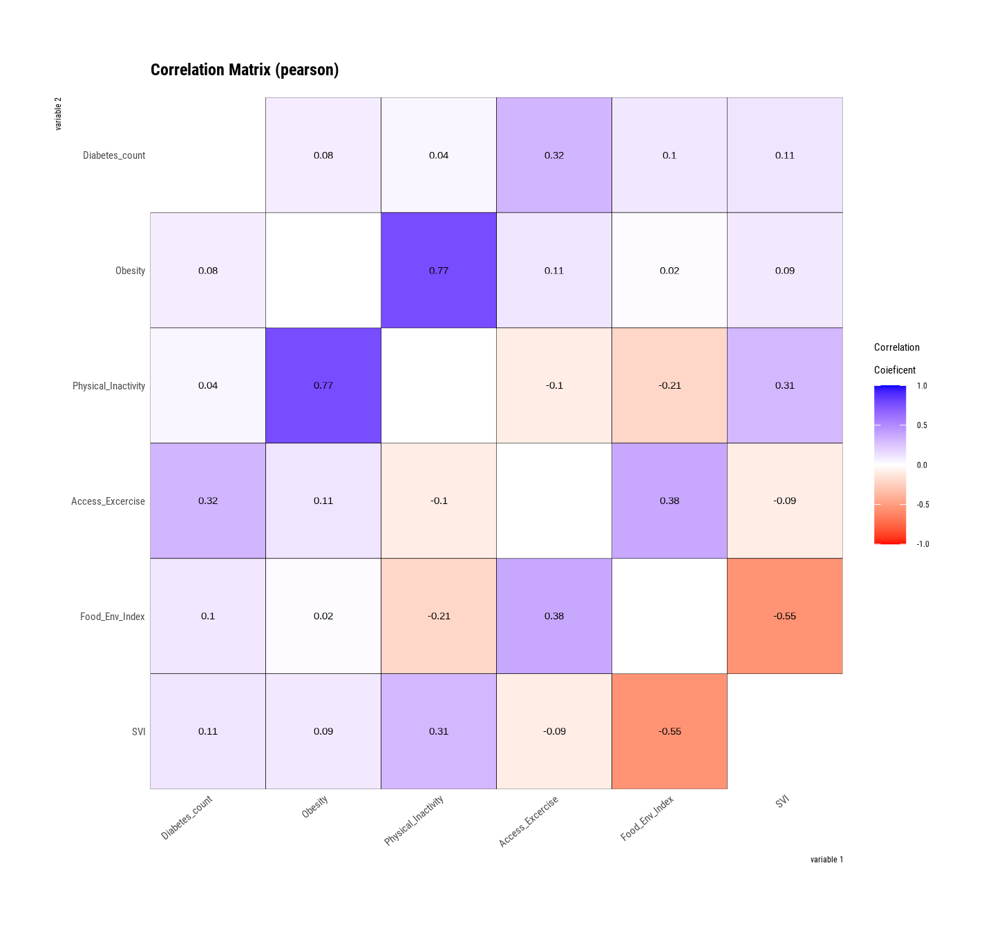
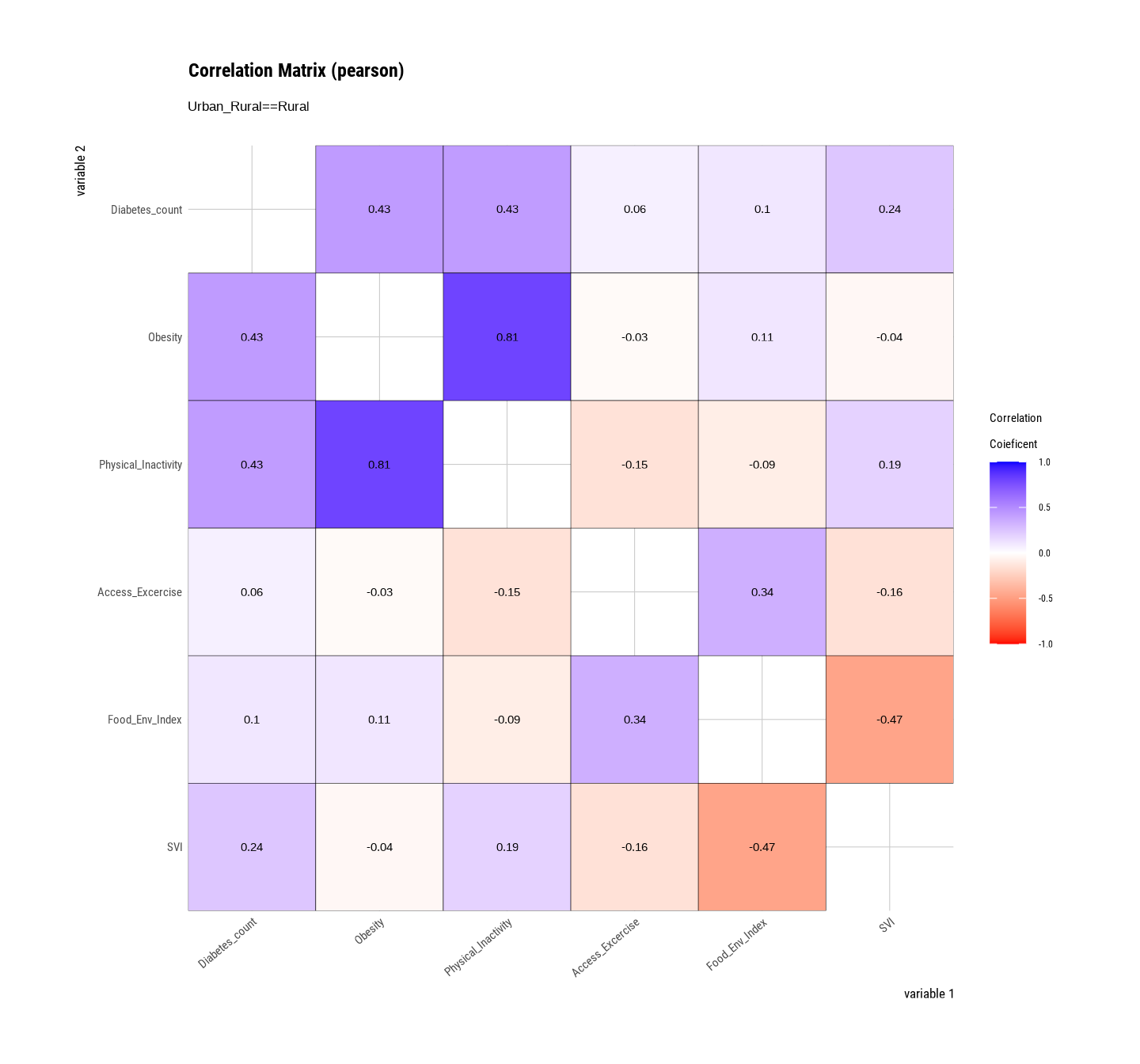
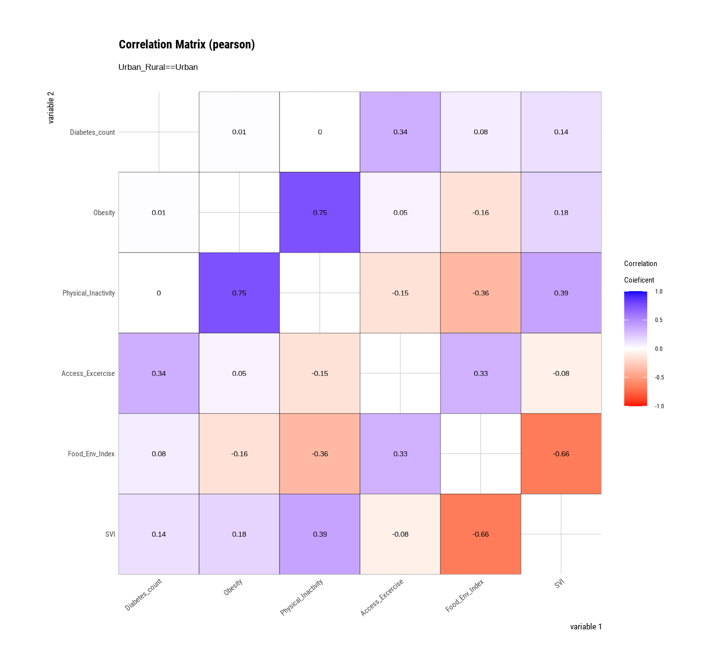
Correlation
plot.correlate() function {dlookr} package visualizes the correlation matrix of a dataframe:
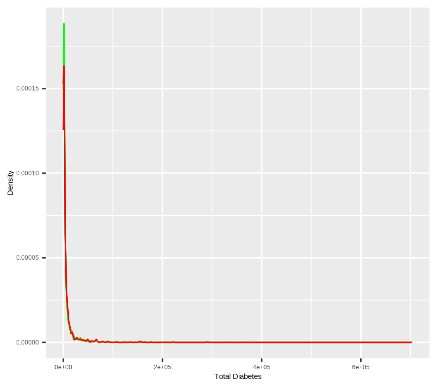
We will use the ddply() function of the {plyr} package to split soil carbon datainto homogeneous subgroups using stratified random sampling. This method involves dividing the population into strata and taking random samples from each stratum to ensure that each subgroup is proportionally represented in the sample. The goal is to obtain a representative sample of the population by adequately representing each stratum.
# Density plot all, train and test data ggplot()+geom_density(data = df, aes(Diabetes_count))+geom_density(data = train, aes(Diabetes_count), color ="green")+geom_density(data = test, aes(Diabetes_count), color ="red") +xlab("Total Diabetes") +ylab("Density")
Fit a standard Poisson Model
We will fit a Poisson regression model using the glm() function in R. We specify family = poisson(link = "log") to indicate that we want to fit a Poisson regression model. Here we model the diabetes rate per county, The offset variable, here is log population per county need to be defined in model. This offset variable adjusts for the differing number of diabetes patients in different population levels per county.
summary() function produce result summaries of the results of model fitting functions.
Code
summary(fit.pois)
Call:
glm(formula = Diabetes_count ~ ., family = poisson(link = "log"),
    data = train)

Coefficients:
                      Estimate Std. Error z value Pr(>|z|)
(Intercept)         -1.518e+00  3.944e-03  -384.8   <2e-16 ***
Obesity              1.073e-02  7.306e-05   146.9   <2e-16 ***
Physical_Inactivity  2.464e-02  8.873e-05   277.7   <2e-16 ***
Access_Excercise     5.281e-02  1.933e-05  2731.9   <2e-16 ***
Food_Env_Index       4.435e-01  3.878e-04  1143.8   <2e-16 ***
SVI                  2.274e+00  1.272e-03  1787.5   <2e-16 ***
Urban_RuralUrban     1.415e+00  1.039e-03  1361.2   <2e-16 ***
---
Signif. codes:  0 '***' 0.001 '**' 0.01 '*' 0.05 '.' 0.1 ' ' 1

(Dispersion parameter for poisson family taken to be 1)

    Null deviance: 44477976  on 2172  degrees of freedom
Residual deviance: 15615853  on 2166  degrees of freedom
AIC: 15636634

Number of Fisher Scoring iterations: 6
The adequacy of a model is typically determined by evaluating the difference between Null deviance and Residual deviance, with a larger discrepancy between the two values indicating a better fit. Null deviance denotes the value obtained when the equation comprises solely the intercept without any variables, while Residual deviance denotes the value calculated when all variables are taken into account. The model can be deemed an appropriate fit when the difference between the two values is substantial enough.
To obtain the AIC (Akaike Information Criterion) values for a GLM model in R, you can use the AIC() function applied to the fitted model. The lower the AIC value, the better the model fits the data while penalizing for the number of parameters. You can compare AIC values between different models to assess their relative goodness-of-fit.
report() function of {report} package generate a brief report of fitted model
Code
report::report(fit.pois)
We fitted a poisson model (estimated using ML) to predict Diabetes_count with
Obesity, Physical_Inactivity, Access_Excercise, Food_Env_Index, SVI and
Urban_Rural (formula: Diabetes_count ~ Obesity + Physical_Inactivity +
Access_Excercise + Food_Env_Index + SVI + Urban_Rural). The model's explanatory
power is substantial (Nagelkerke's R2 = 1.00). The model's intercept,
corresponding to Obesity = 0, Physical_Inactivity = 0, Access_Excercise = 0,
Food_Env_Index = 0, SVI = 0 and Urban_Rural = Rural, is at -1.52 (95% CI
[-1.53, -1.51], p < .001). Within this model:

  - The effect of Obesity is statistically significant and positive (beta = 0.01,
95% CI [0.01, 0.01], p < .001; Std. beta = 0.05, 95% CI [0.05, 0.05])
  - The effect of Physical Inactivity is statistically significant and positive
(beta = 0.02, 95% CI [0.02, 0.02], p < .001; Std. beta = 0.11, 95% CI [0.11,
0.11])
  - The effect of Access Excercise is statistically significant and positive
(beta = 0.05, 95% CI [0.05, 0.05], p < .001; Std. beta = 1.16, 95% CI [1.15,
1.16])
  - The effect of Food Env Index is statistically significant and positive (beta
= 0.44, 95% CI [0.44, 0.44], p < .001; Std. beta = 0.48, 95% CI [0.48, 0.48])
  - The effect of SVI is statistically significant and positive (beta = 2.27, 95%
CI [2.27, 2.28], p < .001; Std. beta = 0.66, 95% CI [0.66, 0.66])
  - The effect of Urban Rural [Urban] is statistically significant and positive
(beta = 1.41, 95% CI [1.41, 1.42], p < .001; Std. beta = 1.41, 95% CI [1.41,
1.42])

Standardized parameters were obtained by fitting the model on a standardized
version of the dataset. 95% Confidence Intervals (CIs) and p-values were
computed using a Wald z-distribution approximation.
The {jtools} package consists of a series of functions to create summary of the poisson regression model:
Code
jtools::summ(fit.pois)
Observations
2173
Dependent variable
Diabetes_count
Type
Generalized linear model
Family
poisson
Link
log
𝛘²(6)
28862122.79
p
0.00
Pseudo-R² (Cragg-Uhler)
1.00
Pseudo-R² (McFadden)
0.65
AIC
15636634.19
BIC
15636673.98
Est.
S.E.
z val.
p
(Intercept)
-1.52
0.00
-384.85
0.00
Obesity
0.01
0.00
146.91
0.00
Physical_Inactivity
0.02
0.00
277.74
0.00
Access_Excercise
0.05
0.00
2731.86
0.00
Food_Env_Index
0.44
0.00
1143.79
0.00
SVI
2.27
0.00
1787.55
0.00
Urban_RuralUrban
1.41
0.00
1361.17
0.00
Standard errors: MLE
We utilized the R package {sandwich} to obtain the robust standard errors and subsequently calculated the p-values. Additionally, we computed the 95% confidence interval using the parameter estimates and their robust standard errors.
Goodness of fit test of poisson can be explored by poisgof() function of {epiDisplay} package:
Code
epiDisplay::poisgof(fit.pois)
$results
[1] "Goodness-of-fit test for Poisson assumption"

$chisq
[1] 15615853

$df
[1] 2166

$p.value
[1] 0
We can generate a report using report() function of {reoprt} package:
Code
report::report(fit.pois)
We fitted a poisson model (estimated using ML) to predict Diabetes_count with
Obesity, Physical_Inactivity, Access_Excercise, Food_Env_Index, SVI and
Urban_Rural (formula: Diabetes_count ~ Obesity + Physical_Inactivity +
Access_Excercise + Food_Env_Index + SVI + Urban_Rural). The model's explanatory
power is substantial (Nagelkerke's R2 = 1.00). The model's intercept,
corresponding to Obesity = 0, Physical_Inactivity = 0, Access_Excercise = 0,
Food_Env_Index = 0, SVI = 0 and Urban_Rural = Rural, is at -1.52 (95% CI
[-1.53, -1.51], p < .001). Within this model:

  - The effect of Obesity is statistically significant and positive (beta = 0.01,
95% CI [0.01, 0.01], p < .001; Std. beta = 0.05, 95% CI [0.05, 0.05])
  - The effect of Physical Inactivity is statistically significant and positive
(beta = 0.02, 95% CI [0.02, 0.02], p < .001; Std. beta = 0.11, 95% CI [0.11,
0.11])
  - The effect of Access Excercise is statistically significant and positive
(beta = 0.05, 95% CI [0.05, 0.05], p < .001; Std. beta = 1.16, 95% CI [1.15,
1.16])
  - The effect of Food Env Index is statistically significant and positive (beta
= 0.44, 95% CI [0.44, 0.44], p < .001; Std. beta = 0.48, 95% CI [0.48, 0.48])
  - The effect of SVI is statistically significant and positive (beta = 2.27, 95%
CI [2.27, 2.28], p < .001; Std. beta = 0.66, 95% CI [0.66, 0.66])
  - The effect of Urban Rural [Urban] is statistically significant and positive
(beta = 1.41, 95% CI [1.41, 1.42], p < .001; Std. beta = 1.41, 95% CI [1.41,
1.42])

Standardized parameters were obtained by fitting the model on a standardized
version of the dataset. 95% Confidence Intervals (CIs) and p-values were
computed using a Wald z-distribution approximation.
Model Performance
performance() function of {performance} package compute indices of model performance for poisson model.
Nagelkerke’s \(R^2\), also known as the Nagelkerke pseudo-\(R^2\), is a measure of the proportion of variance explained by a logistic regression model. It is an adaptation of Cox and Snell’s \(R^2\) to overcome its limitation of having a maximum value less than 1. Nagelkerke’s \(R^2\) ranges from 0 to 1 and provides a measure of the overall fit of the logistic regression model.
Log-Likelihood_model is the log-likelihood of the fitted logistic regression model.
Log-Likelihood_null model is the log-likelihood of the null model (a logistic regression model with only the intercept term).
n is the total number of observations in the dataset.
Nagelkerke’s \(R^2\) provides a useful measure to evaluate the goodness of fit of a logistic regression model, but it should be interpreted with caution, especially when the model has categorical predictors or interactions. Additionally, like other R^2 measures, Nagelkerke’s \(R^2\) does not indicate the quality of predictions made by the model.
Model Diagnostics
The package {performance} provides many functions to check model assumptions, like check_overdispersion(), check_zeroinflation().
Check for Overdispersion
Overdispersion occurs when the observed variance in the data is higher than the expected variance from the model assumption (for Poisson, variance roughly equals the mean of an outcome). check_overdispersion() checks if a count model (including mixed models) is overdispersed or not.
Code
performance::check_overdispersion(fit.pois)
# Overdispersion test

       dispersion ratio =    11872.168
  Pearson's Chi-Squared = 25715115.315
                p-value =      < 0.001
Overdispersion detected.
Overdispersion can be fixed by either modelling the dispersion parameter (not possible with all packages), or by choosing a different distributional family (like Quasi-Poisson, or negative binomial, see (Gelman and Hill 2007)).
Check for Zero-inflation
Zero-inflation (in (Quasi-)Poisson models) is indicated when the amount of observed zeros is larger than the amount of predicted zeros, so the model is underfitting zeros. In such cases, it is recommended to use negative binomial or zero-inflated models.
Use check_zeroinflation() to check if zero-inflation is present in the fitted model.
Code
performance::check_zeroinflation(fit.pois)
Model has no observed zeros in the response variable.
NULL
Check for Singular Model Fits
A “singular” model fit means that some dimensions of the variance-covariance matrix have been estimated as exactly zero. This often occurs for mixed models with overly complex random effects structures.
check_singularity() checks mixed models (of class lme, merMod, glmmTMB or MixMod) for singularity, and returns TRUE if the model fit is singular.
Code
check_singularity(fit.pois)
[1] FALSE
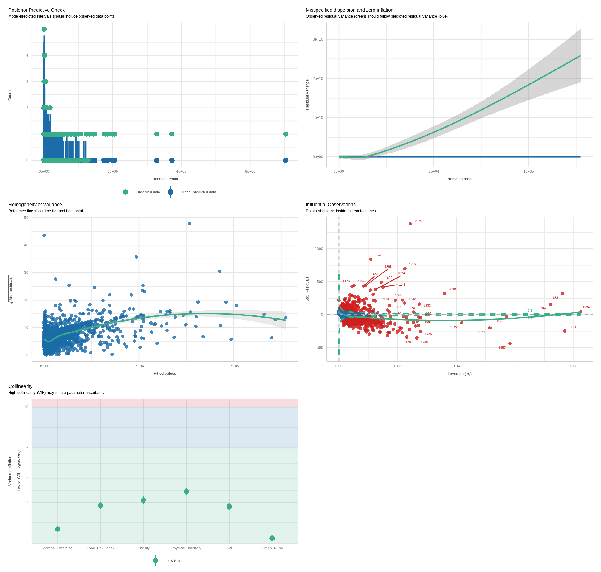
Visualization of Model Assumptions
To get a comprehensive check and visualization, use check_model().
Code
performance::check_model(fit.pois)
Incidence Rate Ratio (IRR)
The Incidence Rate Ratio (IRR) is a measure commonly used in epidemiology and other fields to quantify the association between an exposure or predictor variable and an outcome, particularly when dealing with count data. It is often used in the context of Poisson regression models.
In Poisson regression, the exponentiated coefficients (i.e., exponentiated regression coefficients) are interpreted as Incidence Rate Ratios. Specifically, for a given predictor variable, the IRR represents the multiplicative change in the rate of the outcome for each unit change in the predictor variable.
Mathematically, if \(\beta\) is the coefficient estimate of a predictor variable in a Poisson regression model, then the corresponding IRR, denoted as ( ), is calculated as:
\[ \text{IRR} = e^{\beta} \]
where \(e\) is the base of the natural logarithm (approximately equal to 2.718).
Interpretation of the IRR:
If \(text{IRR} = 1\), it implies that there is no association between the predictor variable and the outcome.
If \(\text{IRR} > 1\), it indicates that an increase in the predictor variable is associated with an increased incidence rate (or risk) of the outcome.
If \(\text{IRR} < 1\), it suggests that an increase in the predictor variable is associated with a decreased incidence rate (or risk) of the outcome.
For example, if the IRR associated with a particular exposure is 1.5, it means that the incidence rate of the outcome is 1.5 times higher in the exposed group compared to the unexposed group, all else being equal.
The IRR provides a convenient way to quantify and interpret the strength of association between predictor variables and outcomes in Poisson regression models, particularly when dealing with count data and incidence rates.
Let’s estimate the IRR value of Obesity, where it coefficient is 0.01073372 . The exponent of this value is:
The tbl_regression() function from the {}* package takes a regression model object as input and produces a formatted table with IRR and confidence interval.
Code
gtsummary::tbl_regression(fit.pois)
Characteristic
log(IRR)
95% CI
p-value
Obesity
0.01
0.01, 0.01
<0.001
Physical_Inactivity
0.02
0.02, 0.02
<0.001
Access_Excercise
0.05
0.05, 0.05
<0.001
Food_Env_Index
0.44
0.44, 0.44
<0.001
SVI
2.3
2.3, 2.3
<0.001
Urban_Rural
Rural
—
—
Urban
1.4
1.4, 1.4
<0.001
Abbreviations: CI = Confidence Interval, IRR = Incidence Rate Ratio
Based on this table, we may interpret the results as follows:
Urban counties have an high number of diabetes with an IRR of 2.38 (95% CI: 2.37, 2.37), while controlling for the effect other variables.
An increase in Obesity one mark increases the risk of having higher number diabetes patients by 0.98 (95% CI: 0.98, 0.98), while while controlling for the effect other variables
Marginal Effects and Adjusted Predictions
If we want the marginal effects for “Obesity”, you may use margins() function of {margins} package:
Code
margins::margins(fit.pois, variables ="Obesity")
Average marginal effects
glm(formula = Diabetes_count ~ ., family = poisson(link = "log"), data = train)
 Obesity
   83.35
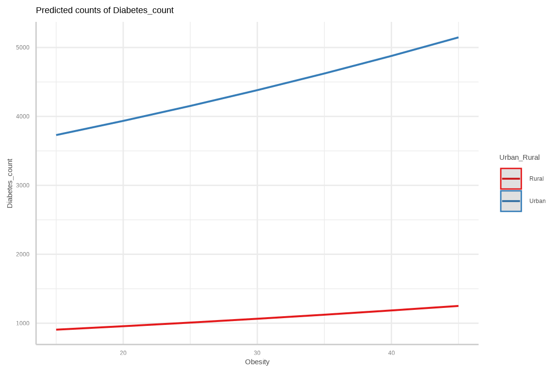
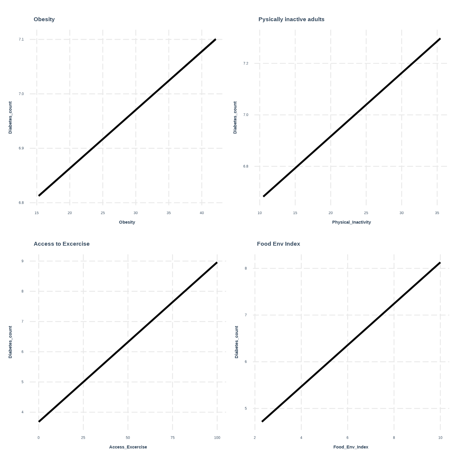
predict_response() function of {ggeffects} calculates predicted count and plot()- method automatically sets titles, axis - and legend-labels depending on the value and variable labels of the data
Code
res <-predict_response(fit.pois, terms =c("Obesity", "Urban_Rural"))res
The predict() function will be used to predict the number of diabetes patients the test counties. This will help to validate the accuracy of the these regression model.
Code
test$Pred.diabetes<-predict(fit.pois, test, type ="response")Metrics::rmse(test$Diabetes_count, test$Pred.diabetes)
Poisson regression is a useful tool for modeling count data, where the response variable represents the number of occurrences of an event. It offers a simple and effective way to analyze the relationship between predictor variables and counts, especially when the event count data follow a Poisson distribution.
In R, you can fit a Poisson regression model using the glm() function. The interpretation of model coefficients is meaningful when we are interested in understanding how predictor variables influence the log of expected counts. However, if overdispersion (where variance exceeds the mean) is detected, alternative models such as Negative Binomial regression may provide better results.
The tutorial covers both the theoretical foundation of Poisson regression and practical steps to implement, evaluate, and interpret it in R, providing users with a solid framework for working with count data in various applications.