Code
# Generate Synthetic Data
set.seed(123)
n <- 100
p <- 10
X <- matrix(rnorm(n * p), n, p)
beta <- c(1, -1, 0, 0.5, -0.5, rep(0, p - 5))
y <- X %*% beta + rnorm(n)![]()

Regularized regression methods are vital for managing high-dimensional datasets or multicollinearity. Techniques like Ridge, Lasso, and Elastic Net add a penalty term to the least squares objective, stabilizing and improving model performance, especially when traditional linear regression risks overfitting. In this tutorial, we will fit Regularized Generalized Linear Models (GLMs) for continuous (Gaussian) data in R. We will start by examining regularization techniques and build models for Ridge, Lasso, and Elastic Net to understand their mathematical foundations. We will then explore the {glmnet} package, which streamlines fitting and cross-validating these models and optimizes the regularization parameter \(\lambda\). We will evaluate each model’s performance using cross-validation and discuss the most suitable contexts for each technique. By the end of this tutorial, you will understand how to implement and interpret regularized GLM models for continuous data in R from both foundational and practical perspectives.
A regularized Generalized Linear Model (GLM) with a Gaussian distribution is essentially a regularized linear regression model. When the response variable ( Y ) follows a Gaussian (normal) distribution, the GLM simplifies to ordinary least squares (OLS) regression. Adding regularization modifies the objective function to penalize the size of the coefficients, aiming to prevent overfitting and improve model interpretability and generalizability.
1. Standard Linear Regression (GLM with Gaussian Distribution)
In a standard linear regression (GLM with a Gaussian distribution):
Random Component: The response variable \(Y\) follows a normal distribution with mean \(\mu\) and variance \(\sigma^2\). \[ Y \sim \mathcal{N}(\mu, \sigma^2) \]
Systematic Component: We assume a linear relationship between predictors and the mean of the response:
\[ \mu = X \ \]
where \(X\) is the matrix of predictors and \(\beta\)) is the vector of coefficients.
Identity Link Function: For Gaussian distributions, the link function \(g(\mu) = \mu\), meaning \(\mathbb{E}[Y] = X \beta\).
The objective function for linear regression is derived by maximizing the likelihood, which is equivalent to minimizing the sum of squared errors (SSE):
\[ \mathcal{L}(\beta) = \sum_{i=1}^n (y_i - X_i \beta)^2 \]
2. Regularized Linear Regression (Regularized Gaussian GLM)
In regularized regression, we add a penalty term to the objective function to control the size of the coefficients ( ). The regularized objective function becomes:
\[ \mathcal{L}_{\text{regularized}}(\beta) = \sum_{i=1}^n (y_i - X_i \beta)^2 + \lambda P \]
where:
- \(\lambda \geq 0\) is the regularization parameter, controlling the amount of penalty.
\(P(\beta)\) is the penalty function. Common choices include:
\[ P(\beta) = \|\beta\|_2^2 =\sum_{j=1}^p \beta_j^2 \]
\[ P(\beta) = \|\beta\|_1 = \sum_{j=1}^p |\beta_j| \]
\[ P(\beta) = \alpha\|\beta\|_1 + (1 - \alpha) \|\beta\|_2^2 \]
which combines L1 and L2 penalties.
Ridge (L2) Regularization:
For Ridge regression, the objective function is: \[ \mathcal{L}_{\text{ridge}}(\beta) = \sum_{i=1}^n (y_i - X_i \beta)^2 + \lambda \sum_{j=1}^p \beta_j^2 \]
The L2 penalty shrinks the coefficients toward zero but does not set them exactly to zero, making it useful for models with many correlated predictors.
Lasso (L1) Regularization:
For Lasso regression, the objective function is: \[ \mathcal{L}_{\text{lasso}}(\beta) = \sum_{i=1}^n (y_i - X_i \beta)^2 + \lambda \sum_{j=1}^p |\beta_j| \]
The L1 penalty encourages sparsity, meaning it tends to set some coefficients exactly to zero, which is useful for feature selection.
Elastic Net Regularization:
For Elastic Net, the objective function is a combination of both L1 and L2 penalties:
\[ \mathcal{L}_{\text{elastic net}}(\beta) = \sum_{i=1}^n (y_i - X_i \beta)^2 + \lambda \left( \alpha \sum_{j=1}^p |\beta_j| + (1 - \alpha) \sum_{j=1}^p \beta_j^2 \right) \]
Elastic Net allows you to balance between Lasso and regularization, providing both feature selection and coefficient shrinkage.
Optimization
The coefficients \(\beta\) are estimated by minimizing the regularized objective function with respect to \(\beta\). Depending on the penalty, different optimization techniques are used:
To perform regularized regression (Ridge, Lasso, and Elastic Net) on synthetic data in R without using any libraries, we need to manually implement each regularization method in the GLM framework. Here’s how to proceed:
Create synthetic data using the following code:
# Generate Synthetic Data
set.seed(123)
n <- 100
p <- 10
X <- matrix(rnorm(n * p), n, p)
beta <- c(1, -1, 0, 0.5, -0.5, rep(0, p - 5))
y <- X %*% beta + rnorm(n)Next, we implement the coordinate descent algorithm to solve the regularized regression problem. The algorithm iteratively updates each coefficient by minimizing the objective function with respect to that coefficient while keeping the others fixed. The update rule depends on the type of regularization (Ridge, Lasso, or Elastic Net). Here’s the implementation in R:
#  Coordinate Descent Algorithm
coordinate_descent <- function(X, y, lambda, alpha, tol = 1e-6, max_iter = 1000) {
  n <- nrow(X)
  p <- ncol(X)
  beta <- rep(0, p)
  X <- scale(X)  # Standardize features
  y <- y - mean(y)  # Center target

  for (iter in 1:max_iter) {
    beta_old <- beta
    for (j in 1:p) {
      r_j <- y - X %*% beta + beta[j] * X[, j]
      z_j <- sum(X[, j]^2)
      rho_j <- sum(X[, j] * r_j)

      # Update beta based on the type of model (Ridge, Lasso, ElasticNet)
      beta[j] <- ifelse(alpha == 1, # Lasso
                        sign(rho_j) * max(abs(rho_j) - lambda, 0) / z_j,
                        ifelse(alpha == 0, # Ridge
                               rho_j / (z_j + lambda),
                               # Elastic Net
                               sign(rho_j) * max(abs(rho_j) - lambda * alpha, 0) / (z_j + lambda * (1 - alpha))))
    }
    if (sum(abs(beta - beta_old)) < tol) break
  }
  return(beta)
}We can perform cross-validation to select the best hyperparameters (alpha and lambda) for the regularized regression model. This involves splitting the data into k folds, training the model on k-1 folds, and evaluating it on the remaining fold. We repeat this process for different values of alpha and lambda to find the best combination. Here’s how to implement cross-validation in R:
# Cross-Validation for Hyperparameter Tuning (including alpha)
cv_glm <- function(X, y, alpha_seq, lambda_seq, k = 5) {
  n <- nrow(X)
  folds <- sample(1:k, n, replace = TRUE)
  best_mse <- Inf
  best_lambda <- NULL
  best_alpha <- NULL

  for (alpha in alpha_seq) {
    mse_vals <- numeric(length(lambda_seq))

    for (i in seq_along(lambda_seq)) {
      lambda <- lambda_seq[i]
      fold_errors <- numeric(k)

      # Cross-validation for each fold
      for (fold in 1:k) {
        X_train <- X[folds != fold, ]
        y_train <- y[folds != fold]
        X_val <- X[folds == fold, ]
        y_val <- y[folds == fold]

        beta <- coordinate_descent(X_train, y_train, lambda, alpha)
        y_pred <- X_val %*% beta
        fold_errors[fold] <- mean((y_val - y_pred)^2)
      }
      mse_vals[i] <- mean(fold_errors)
    }

    # Find the best lambda for the current alpha
    min_mse <- min(mse_vals)
    if (min_mse < best_mse) {
      best_mse <- min_mse
      best_lambda <- lambda_seq[which.min(mse_vals)]
      best_alpha <- alpha
    }
  }

  return(list(best_alpha = best_alpha, best_lambda = best_lambda))
}Finally, we can train the regularized regression models for all alpha values (0 for Ridge, 0.5 for Elastic Net, and 1 for Lasso) and select the best alpha and lambda based on cross-validation results. We then fit the final model using the best hyperparameters and evaluate its performance. Here’s how to implement this in R:
# Standardize X for better regularization performance
X_scaled <- scale(X)

# Train Models for All Alpha Values
alpha_values <- c(0, 0.5, 1)  # Ridge (0), ElasticNet (0.5), Lasso (1)
lambda_seq <- 10^seq(-3, 1, length.out = 50)

# Find the best alpha and lambda
cv_results <- cv_glm(X_scaled, y, alpha_values, lambda_seq, k = 5)

# Best alpha and lambda
best_alpha <- cv_results$best_alpha
best_lambda <- cv_results$best_lambda

# Train the final model using the best alpha and lambda
final_beta <- coordinate_descent(X_scaled, y, best_lambda, best_alpha)
y_pred <- X_scaled %*% final_beta

# Calculate performance metrics
mse <- mean((y - y_pred)^2)
r_squared <- 1 - sum((y - y_pred)^2) / sum((y - mean(y))^2)

cat("\nFinal Model (Best Alpha =", best_alpha, "and Lambda =", best_lambda, "):\n")
Final Model (Best Alpha = 1 and Lambda = 1.84207 ):cat("MSE:", mse, "\n")MSE: 1.025086 cat("R-squared:", r_squared, "\n")R-squared: 0.7275239 # Visualize Coefficients
library(ggplot2)
coef_df <- data.frame(
Feature = 1:ncol(X),
Coefficients = final_beta
)
ggplot(coef_df, aes(x = Feature, y = Coefficients)) +
geom_point() +
geom_line() +
labs(title = paste("Coefficients (Best Alpha =", best_alpha, ")"), x = "Feature", y = "Coefficient") +
theme_minimal()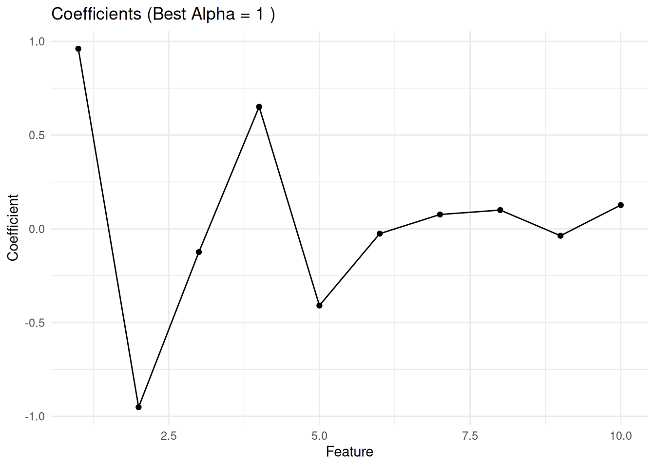
Fit Ridge, Lasso, and Elastic Net models:
# Fit Ridge, Lasso, and Elastic Net models
ridge_beta <- coordinate_descent(X_scaled, y, lambda = best_lambda, alpha = 0)
lasso_beta <- coordinate_descent(X_scaled, y, lambda = best_lambda, alpha = 1)
elastic_net_beta <- coordinate_descent(X_scaled, y, lambda = best_lambda, alpha = best_alpha)

# Combine coefficients into a data frame
coef_summary <- data.frame(
  Predictor = paste0("X", 1:10),
  Ridge = round(ridge_beta, 3),
  Lasso = round(lasso_beta , 3),
  Elastic_Net = round(elastic_net_beta, 3)

)

print(coef_summary)
Predictor Ridge Lasso Elastic_Net
1 X1 0.954 0.961 0.961
2 X2 -0.951 -0.951 -0.951
3 X3 -0.140 -0.124 -0.124
4 X4 0.646 0.651 0.651
5 X5 -0.416 -0.409 -0.409
6 X6 -0.042 -0.026 -0.026
7 X7 0.090 0.077 0.077
8 X8 0.117 0.100 0.100
9 X9 -0.053 -0.037 -0.037
10 X10 0.143 0.127 0.127# Predicted values for each model
y_pred_ridge <- X_scaled %*% ridge_beta
y_pred_lasso <- X_scaled %*% lasso_beta
y_pred_elastic_net <- X_scaled %*% elastic_net_betacalculate_metrics <- function(observed, predicted) {
# Ensure inputs are numeric vectors
observed <- as.numeric(observed)
predicted <- as.numeric(predicted)
# Compute metrics
mse <- mean((observed - predicted)^2)
rmse <- sqrt(mse)
mae <- mean(abs(observed - predicted))
medae <- median(abs(observed - predicted))
r2 <- 1 - sum((observed - predicted)^2) / sum((observed - mean(observed))^2)
# Return results as a named list
metrics <- list(
RMSE = rmse,
MAE = mae,
MSE = mse,
MedAE = medae,
R2 = r2
)
return(metrics)
}# Evaluate Ridge model
calculate_metrics(y, y_pred_ridge)$RMSE
[1] 1.011627
$MAE
[1] 0.7968189
$MSE
[1] 1.02339
$MedAE
[1] 0.6705467
$R2
[1] 0.7279747# Evaluate Lasso model
calculate_metrics(y, y_pred_lasso)$RMSE
[1] 1.012465
$MAE
[1] 0.7986907
$MSE
[1] 1.025086
$MedAE
[1] 0.6622258
$R2
[1] 0.7275239# Evaluate Elastic Net model
calculate_metrics(y,y_pred_elastic_net)$RMSE
[1] 1.012465
$MAE
[1] 0.7986907
$MSE
[1] 1.025086
$MedAE
[1] 0.6622258
$R2
[1] 0.7275239To fit a Regularized Generalized Linear Model (GLM) with a Gaussian distribution (equivalent to linear regression) in R, we will use {glmnet} package.
Following R packages are required to run this notebook. If any of these packages are not installed, you can install them using the code below:
packages <- c('tidyverse',
     'plyr',
         'ggpmisc',
         'rstatix',
         'ggeffects',
         'patchwork',
         #'metrica',
         'Metrics',
         'ggpmisc',
         'glmnet'
        )
#| warning: false
#| error: false
# Install missing packages
new_packages <- packages[!(packages %in% installed.packages()[,"Package"])]
if(length(new_packages)) install.packages(new_packages)
# Verify installation
cat("Installed packages:\n")
print(sapply(packages, requireNamespace, quietly = TRUE))# Load packages with suppressed messages
invisible(lapply(packages, function(pkg) {
suppressPackageStartupMessages(library(pkg, character.only = TRUE))
}))# Check loaded packages
cat("Successfully loaded packages:\n")Successfully loaded packages:print(search()[grepl("package:", search())]) [1] "package:glmnet" "package:Matrix" "package:Metrics"
[4] "package:patchwork" "package:ggeffects" "package:rstatix"
[7] "package:ggpmisc" "package:ggpp" "package:plyr"
[10] "package:lubridate" "package:forcats" "package:stringr"
[13] "package:dplyr" "package:purrr" "package:readr"
[16] "package:tidyr" "package:tibble" "package:tidyverse"
[19] "package:ggplot2" "package:stats" "package:graphics"
[22] "package:grDevices" "package:utils" "package:datasets"
[25] "package:methods" "package:base" Our goal is to develop a GLM regression model to predict paddy soil arsenic (SAs) concentration using various irrigation water and soil properties. We have available data of 263 paired groundwater and paddy soil samples from arsenic contaminated areas in Tala Upazilla, Satkhira district, Bangladesh. This data was utilized in a publication titled “Factors Affecting Paddy Soil Arsenic Concentration in Bangladesh: Prediction and Uncertainty of Geostatistical Risk Mapping” which can be accessed via the this URL
Full data set is available for download from my Dropbox or from my Github accounts.
We will use read_csv() function of readr package to import data as a tidy data.
# Load data
mf<-read_csv("https://github.com/zia207/r-colab/raw/main/Data/Regression_analysis/bd_soil_arsenic.csv")df <- mf |>
# select variables
dplyr::select (WAs, WP, WFe,
WEc, WpH, SAoFe, SpH, SOC,
Sand, Silt, SP, Elevation,
Year_Irrigation, Distance_STW,
Land_type, SAs) |>
# convert to factor
dplyr::mutate_at(vars(Land_type), funs(factor)) |>
# create a variable
dplyr::mutate (Silt_Sand = Silt+Sand) |>
# drop two variables
dplyr::select(-c(Silt,Sand)) |>
# relocate or organized variable
dplyr::relocate(SAs, .after=Silt_Sand) |>
dplyr::relocate(Land_type, .after=Silt_Sand) |>
# normalize the all numerical features
# dplyr::mutate_at(1:13, funs((.-min(.))/max(.-min(.)))) |>
glimpse()Rows: 263
Columns: 15
$ WAs <dbl> 0.059, 0.059, 0.079, 0.122, 0.072, 0.042, 0.075, 0.064…
$ WP <dbl> 0.761, 1.194, 1.317, 1.545, 0.966, 1.058, 0.868, 0.890…
$ WFe <dbl> 3.44, 4.93, 9.70, 8.58, 4.78, 6.95, 7.81, 8.14, 8.99, …
$ WEc <dbl> 1.03, 1.07, 1.40, 0.83, 1.42, 1.82, 1.71, 1.74, 1.57, …
$ WpH <dbl> 7.03, 7.06, 6.84, 6.85, 6.95, 6.89, 6.86, 6.98, 6.82, …
$ SAoFe <dbl> 2500, 2670, 2160, 2500, 2060, 2500, 2520, 2140, 2150, …
$ SpH <dbl> 7.74, 7.87, 8.03, 8.07, 7.81, 7.77, 7.66, 7.89, 8.00, …
$ SOC <dbl> 1.66, 1.26, 1.36, 1.61, 1.26, 1.74, 1.71, 1.69, 1.41, …
$ SP <dbl> 13.79, 15.31, 15.54, 16.28, 14.20, 13.41, 13.26, 14.84…
$ Elevation <dbl> 3, 5, 4, 3, 5, 2, 2, 3, 3, 3, 2, 5, 6, 6, 5, 5, 4, 6, …
$ Year_Irrigation <dbl> 14, 20, 10, 8, 10, 9, 8, 10, 8, 2, 20, 4, 15, 10, 5, 4…
$ Distance_STW <dbl> 5, 6, 5, 8, 5, 5, 10, 8, 10, 8, 5, 5, 9, 5, 10, 10, 12…
$ Silt_Sand <dbl> 61.1, 59.8, 58.7, 56.3, 63.0, 60.3, 60.2, 54.5, 57.5, …
$ Land_type <fct> MHL, MHL, MHL, MHL, MHL, MHL, MHL, MHL, MHL, MHL, MHL,…
$ SAs <dbl> 29.10, 45.10, 23.20, 23.80, 26.00, 25.60, 26.30, 31.60…We will use the ddply() function of the plyr package to split soil carbon datainto homogeneous subgroups using stratified random sampling. This method involves dividing the population into strata and taking random samples from each stratum to ensure that each subgroup is proportionally represented in the sample. The goal is to obtain a representative sample of the population by adequately representing each stratum.
seeds = 11076
tr_prop = 0.70
# training data (70% data)
train= ddply(df,.(Land_type),
                 function(., seed) { set.seed(seed); .[sample(1:nrow(.), trunc(nrow(.) * tr_prop)), ] }, seed = 101)
test = ddply(df, .(Land_type),
function(., seed) { set.seed(seed); .[-sample(1:nrow(.), trunc(nrow(.) * tr_prop)), ] }, seed = 101)Stratified random sampling Stratified random sampling is a technique for selecting a representative sample from a population, where the sample is chosen in a way that ensures that certain subgroups within the population are adequately represented in the sample.
You need to create two objects:
y for storing the outcome variablex for holding the predictor variables. This should be created using the function model.matrix() allowing to automatically transform any qualitative variables (if any) into dummy variables, which is important because glmnet() can only take numerical, quantitative inputs. After creating the model matrix, we remove the intercept component at index = 1.# Predictor variables
x.train <- model.matrix(SAs~., train)[,-1]
# Outcome variable
y.train <-train$SAs::: callout-note use model.matrix() when you get “error in evaluating the argument ‘x’ in selecting a method for function ‘as.matrix’”. For some reason glmnet prefers data.matrix() to as.matrix() :::
Now we can apply cv.glmnet() function for cross-validation to choose the best lambda (regularization parameter). For example, suppose we designate \(α\)=0 for ridge regression and specify nlambda as 200. This implies that the model fit will be calculated solely for 200 \(λ\) values.
# cross validation
ridge.cv <- cv.glmnet(x= x.train,
                       y= y.train,
                       type.measure="mse",
                       nfold = 5,
                       alpha=0,
                       family="gaussian",
                       nlambda=200,
                       standardize = TRUE)
Printing the resulting object gives some basic information on the cross-validation performed:
print(ridge.cv)
Call:  cv.glmnet(x = x.train, y = y.train, type.measure = "mse", nfolds = 5,      alpha = 0, family = "gaussian", nlambda = 200, standardize = TRUE)

Measure: Mean-Squared Error

    Lambda Index Measure    SE Nonzero
min  1.376   173   28.02 3.055      14
1se  7.988   135   30.99 4.543      14
We can plot ridge.cv object to see how each tested lambda value performed:
plot(ridge.cv)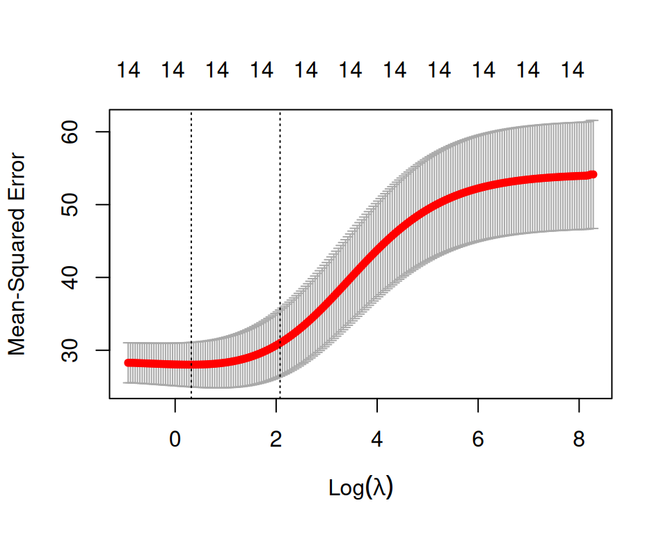
On the graph, the x-axis represents the logarithm of \(λ\), and the y-axis shows the mean-squared error (MSE). A lower MSE indicates a better fit. The graph highlights two specific \(λ\) values with dotted vertical lines. The first value, lambda.min, resulted in the lowest mean-squared error. The second value, called lambda.1se, represents the most considerable \(λ\) value that provides cross-validated error within one standard error of the minimum. Generally, lambda.1se is more important than lambda.min because its goal is to prevent over-fitting. Therefore, we will sacrifice some goodness of fit for greater regularization.
Now, we will extract thelambda.1se with lowest MSE:
# Choose lambda with standard error of the minimum
ridge.cv$lambda.1se
[1] 7.987695Now Fit the final model with the best “lambda”:
# fit ridge regression
ridge.fit <-  glmnet(x= x.train,
                       y= y.train,
                       alpha=0,
                       lambda = ridge.cv$lambda.1se,
                       family="gaussian",
                       nlambda=200,
                       standardize = TRUE)
Printing the resulting object gives some basic information on glmnet() function performed:
print(ridge.fit)
Call:  glmnet(x = x.train, y = y.train, family = "gaussian", alpha = 0,      nlambda = 200, lambda = ridge.cv$lambda.1se, standardize = TRUE)

  Df  %Dev Lambda
1 14 47.43  7.988
The output includes the call that generated the ridge.fit object. Additionally, it displays a three-column matrix containing the following columns: Df (the number of nonzero coefficients), %dev (the percentage of deviance explained), and Lambda (the corresponding value of \(λ\)). You can use the digits parameter to specify the number of significant digits in the printed output.
Finally we will extract the coefficients for the selected \(λ\) using coef() function:
coef(ridge.fit)15 x 1 sparse Matrix of class "dgCMatrix"
s0
(Intercept) 13.2099725762
WAs 6.7164555611
WP 0.3804027472
WFe 0.3493429629
WEc 0.3119772753
WpH -0.1169126885
SAoFe -0.0005835623
SpH 0.3508412746
SOC 1.6901302632
SP 0.0659128651
Elevation -0.3067938115
Year_Irrigation 0.3843561522
Distance_STW -0.0804925909
Silt_Sand -0.0759818371
Land_typeMHL 1.9065149235Now, we will test this model on our test dataset by calculating the model-predicted values for the test dataset and then computing the MAE, MSE, RMSE and R-square:
# Make predictions on the test data
x.test <- model.matrix(SAs ~., test)[,-1]
y.test <-test$SAs

ridge.SAs<-ridge.fit  |>
  predict(x.test)  |>  as.vector()
ridge.pred<-as.data.frame(cbind("Obs_SAs" = y.test, "Pred_SAs"=ridge.SAs))
glimpse(ridge.pred)
Rows: 80
Columns: 2
$ Obs_SAs <dbl> 11.30, 17.10, 11.70, 13.60, 19.80, 14.80, 15.10, 17.20, 10.00…
$ Pred_SAs <dbl> 16.35673, 13.98615, 14.29528, 16.00968, 16.51516, 17.19274, 1…# Model performance metrics
calculate_metrics(ridge.pred$Obs_SAs, ridge.pred$Pred_SAs)$RMSE
[1] 5.953786
$MAE
[1] 4.018209
$MSE
[1] 35.44757
$MedAE
[1] 3.172252
$R2
[1] 0.3729436We can plot observed and predicted values with fitted regression line with ggplot2
formula<-y~x
# Lasso regression
p1=ggplot(ridge.pred, aes(Obs_SAs,Pred_SAs)) +
  geom_point() +
  geom_smooth(method = "lm")+
  stat_poly_eq(use_label(c("eq", "adj.R2")), formula = formula) +
  ggtitle("Ridge Regression ") +
  xlab("Observed") + ylab("Predicted") +
  scale_x_continuous(limits=c(0,60), breaks=seq(0, 60, 10))+
  scale_y_continuous(limits=c(0,60), breaks=seq(0, 60, 10)) +
  theme(
    panel.background = element_rect(fill = "grey95",colour = "gray75",size = 0.5, linetype = "solid"),
    axis.line = element_line(colour = "grey"),
    plot.title = element_text(size = 14, hjust = 0.5),
    axis.title.x = element_text(size = 14),
    axis.title.y = element_text(size = 14),
    axis.text.x=element_text(size=13, colour="black"),
    axis.text.y=element_text(size=13,angle = 90,vjust = 0.5, hjust=0.5, colour='black'))
print(p1)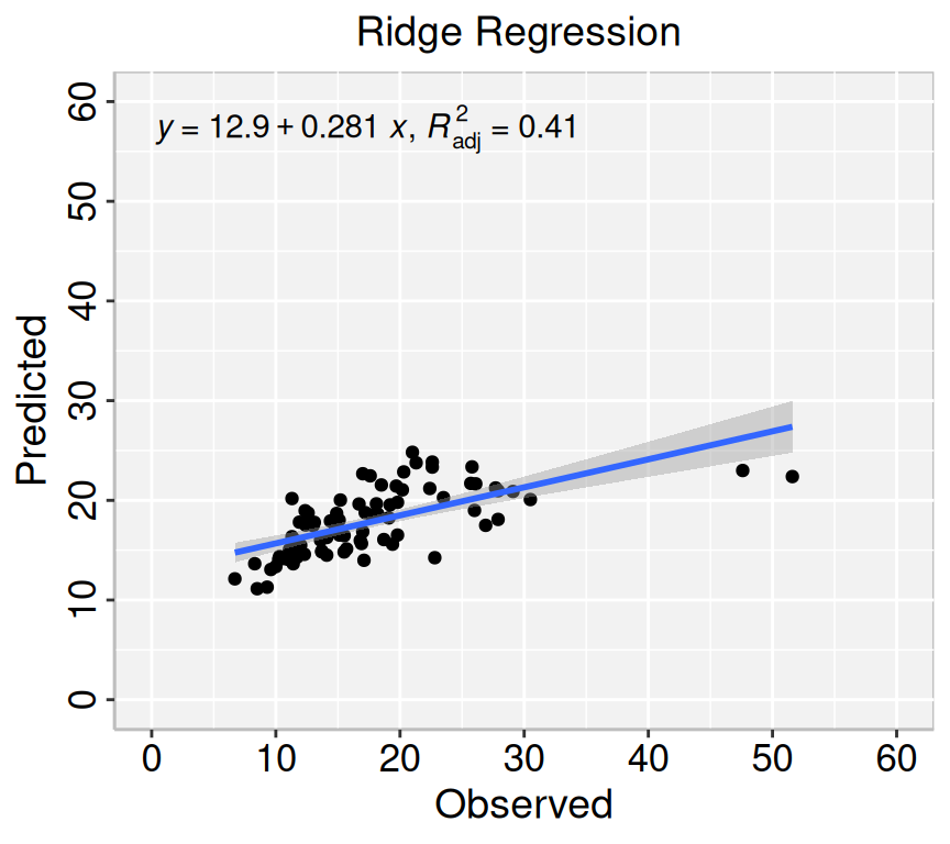
We can set up our model very similarly to our ridge function. We simply need to change the alpha argument to 1 and do K-fold cross-validation:
# cross validation
lasso.cv <- cv.glmnet(x= x.train,
                       y= y.train,
                       type.measure="mse",
                       nfold = 5,
                       alpha=1,
                       family="gaussian",
                       nlambda=200,
standardize = TRUE)print(lasso.cv)
Call:  cv.glmnet(x = x.train, y = y.train, type.measure = "mse", nfolds = 5,      alpha = 1, family = "gaussian", nlambda = 200, standardize = TRUE)

Measure: Mean-Squared Error

    Lambda Index Measure    SE Nonzero
min 0.2343    62   27.91 2.482      11
1se 0.7452 37 30.25 2.741 9plot(lasso.cv)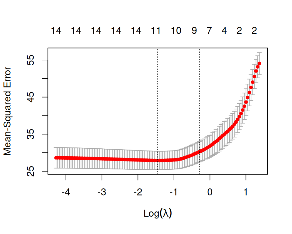
# Choose lambda with standard error of the minimum
lasso.cv$lambda.1se
[1] 0.7451964Now Fit the final model with the best “lambda”:
# fit lasso regression
lasso.fit <-  glmnet(x= x.train,
                       y= y.train,
                       alpha=1,
                       lambda = lasso.cv$lambda.1se,
                       family="gaussian",
                       nlambda=200,
standardize = TRUE)print(lasso.fit)
Call:  glmnet(x = x.train, y = y.train, family = "gaussian", alpha = 1,      nlambda = 200, lambda = lasso.cv$lambda.1se, standardize = TRUE)

  Df  %Dev Lambda
1  9 49.65 0.7452
Finally we will extract the coefficients for the selected \(λ\) using coef() function:
coef(lasso.fit)15 x 1 sparse Matrix of class "dgCMatrix"
s0
(Intercept) 13.13129121
WAs 6.43205983
WP .
WFe 0.31947153
WEc .
WpH .
SAoFe .
SpH .
SOC 0.48232833
SP 0.01443477
Elevation -0.10987428
Year_Irrigation 0.64081854
Distance_STW -0.02963625
Silt_Sand -0.07096227
Land_typeMHL 3.24183879Now, we will test this model on our test dataset by calculating the model-predicted values for the test dataset and then computing the RMSE and R-square:
# Make predictions on the test data
x.test <- model.matrix(SAs ~., test)[,-1]
y.test <-test$SAs

lasso.SAs<-lasso.fit  |>
  predict(x.test)  |>  as.vector()
lasso.pred<-as.data.frame(cbind("Obs_SAs" = y.test, "Pred_SAs"=lasso.SAs))
glimpse(lasso.pred)
Rows: 80
Columns: 2
$ Obs_SAs <dbl> 11.30, 17.10, 11.70, 13.60, 19.80, 14.80, 15.10, 17.20, 10.00…
$ Pred_SAs <dbl> 14.81875, 12.92237, 13.27538, 14.81378, 16.53555, 13.81663, 1…# Model performance metrics
calculate_metrics(lasso.pred$Obs_SAs, lasso.pred$Pred_SAs)$RMSE
[1] 5.774528
$MAE
[1] 3.989926
$MSE
[1] 33.34517
$MedAE
[1] 3.178921
$R2
[1] 0.4101343We can plot observed and predicted values with fitted regression line with ggplot2
formula<-y~x
# Lasso regression
p2=ggplot(lasso.pred, aes(Obs_SAs,Pred_SAs)) +
  geom_point() +
  geom_smooth(method = "lm")+
  stat_poly_eq(use_label(c("eq", "adj.R2")), formula = formula) +
  ggtitle("Lasso Regression ") +
  xlab("Observed") + ylab("Predicted") +
  scale_x_continuous(limits=c(0,60), breaks=seq(0, 60, 10))+
  scale_y_continuous(limits=c(0,60), breaks=seq(0, 60, 10)) +
  theme(
    panel.background = element_rect(fill = "grey95",colour = "gray75",size = 0.5, linetype = "solid"),
    axis.line = element_line(colour = "grey"),
    plot.title = element_text(size = 14, hjust = 0.5),
    axis.title.x = element_text(size = 14),
    axis.title.y = element_text(size = 14),
    axis.text.x=element_text(size=13, colour="black"),
    axis.text.y=element_text(size=13,angle = 90,vjust = 0.5, hjust=0.5, colour='black'))
print(p2)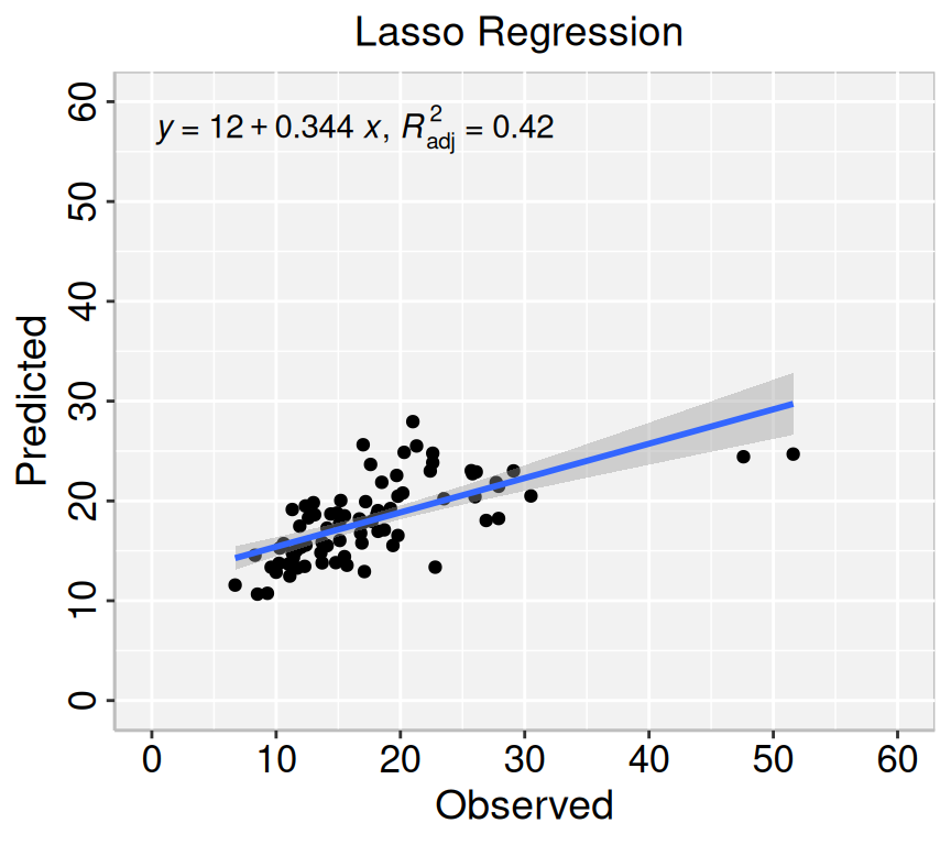
Elastic Net regression is a combination of L1 (LASSO) and L2 (Ridge) regularization. It provides a balance between feature selection and coefficient shrinkage. The glmnet package in R provides efficient functions for fitting Elastic Net regression models.
We can set up our model very similarly to our ridge function. We simply need to change the alphaargument to a value between 0 and 1 and do K-fold cross-validation:
# Define alpha values for Lasso, Ridge, and Elastic Net
alpha_values <- seq(0, 1, by = 0.1)

# Lambda will be generated automatically, but you can also define it manually:
lambda_values <- 10^seq(-4, 1, length.out = 100) # Logarithmic scale

# Cross-validation
results <- list()
for (alpha in alpha_values) {
  cv_model <- cv.glmnet(
    x = x.train,
    y = y.train,
    alpha = alpha,
    lambda = lambda_values,
    nfolds = 5, # 5-fold cross-validation
    standardize = TRUE # Standardizes the predictors by default
  )

  # Store results
  results[[paste("alpha=", alpha)]] <- list(
    alpha = alpha,
    best_lambda = cv_model$lambda.min,
    cv_model = cv_model
  )
}

best_result <- NULL
min_mse <- Inf

for (res in results) {
  mse <- min(res$cv_model$cvm) # Mean squared error
  if (mse < min_mse) {
    min_mse <- mse
    best_result <- res
  }
}

# Best model
cat("Best alpha:", best_result$alpha, "\n")
Best alpha: 0.4 cat("Best lambda:", best_result$best_lambda, "\n")Best lambda: 0.4862602 enet.fit <- glmnet(
x = x.train,
y = y.train,
alpha = best_result$alpha,
lambda = best_result$best_lambda,
standardize = TRUE
)Now, we will test this model on our test dataset by calculating the model-predicted values for the test dataset
# Make predictions on the test data
x.test <- model.matrix(SAs ~., test)[,-1]
y.test <-test$SAs

enet.SAs<-enet.fit  |>
  predict(x.test)  |>  as.vector()
enet.pred<-as.data.frame(cbind("Obs_SAs" = y.test, "Pred_SAs"=ridge.SAs))
glimpse(enet.pred)
Rows: 80
Columns: 2
$ Obs_SAs <dbl> 11.30, 17.10, 11.70, 13.60, 19.80, 14.80, 15.10, 17.20, 10.00…
$ Pred_SAs <dbl> 16.35673, 13.98615, 14.29528, 16.00968, 16.51516, 17.19274, 1…# Model performance metrics
calculate_metrics(enet.pred$Obs_SAs, enet.pred$Pred_SAs)$RMSE
[1] 5.953786
$MAE
[1] 4.018209
$MSE
[1] 35.44757
$MedAE
[1] 3.172252
$R2
[1] 0.3729436We can plot observed and predicted values with fitted regression line with ggplot2
formula<-y~x
# Lasso regression
p3=ggplot(enet.pred, aes(Obs_SAs,Pred_SAs)) +
  geom_point() +
  geom_smooth(method = "lm")+
  stat_poly_eq(use_label(c("eq", "adj.R2")), formula = formula) +
  ggtitle("Elastic Net Regression ") +
  xlab("Observed") + ylab("Predicted") +
  scale_x_continuous(limits=c(0,60), breaks=seq(0, 60, 10))+
  scale_y_continuous(limits=c(0,60), breaks=seq(0, 60, 10)) +
  theme(
    panel.background = element_rect(fill = "grey95",colour = "gray75",size = 0.5, linetype = "solid"),
    axis.line = element_line(colour = "grey"),
    plot.title = element_text(size = 14, hjust = 0.5),
    axis.title.x = element_text(size = 14),
    axis.title.y = element_text(size = 14),
    axis.text.x=element_text(size=13, colour="black"),
    axis.text.y=element_text(size=13,angle = 90,vjust = 0.5, hjust=0.5, colour='black'))
print(p3)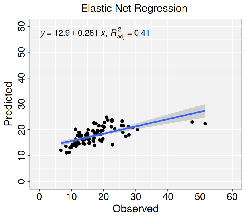
Regularized linear regression (GLM with a Gaussian distribution) helps prevent overfitting by shrinking the coefficient estimates, which can lead to simpler, more interpretable models. The choice of regularization method (L1, L2, or Elastic Net) depends on whether you need feature selection (L1), smoothness (L2), or a balance of both (Elastic Net). Although these methods may seem similar, they have significant differences. Ridge regression uses the square of the coefficients as a penalty, while Lasso regression uses the absolute value of the coefficients. Elastic Net regression combines the penalties of both Ridge and Lasso regression.
This tutorial explored how to implement Regularized Linear Models (GLMs) in R using {glmnet}. Regularized GLMs, such as LASSO, Ridge, and Elastic Net, are essential techniques in predictive modeling, especially when dealing with high-dimensional data or collinear predictors.
To summarize, each package has advantages and capabilities for implementing regularized GLMs in R. factors such as the dataset size, desired modeling workflow, and personal preference should be considered when choosing a package. By mastering these packages, researchers and data scientists can effectively use regularized GLMs for predictive modeling tasks, extracting valuable insights from complex datasets while mitigating overfitting and improving generalization performance.