Gamma regression is a powerful statistical method for modeling positive, continuous data with a skewed distribution, particularly when variability increases with the mean. It is commonly used in insurance claims, healthcare costs, and rainfall data, where values are non-negative and right-skewed. This tutorial will explore Gamma regression in R through two main approaches. First, we will manually build a Gamma regression model to understand its underlying mechanics, including the log-likelihood function and parameter optimization. Then, we will utilize R’s built-in lm () function to simplify the modeling process and demonstrate practical result interpretation. By the end of this tutorial, you will understand how to apply Gamma regression to real-world data by coding from scratch and using R’s built-in functions.
Overview
Gamma regression is used for modeling positive, continuous data where the variance increases with the mean. It assumes that the response variable \(y\) follows a Gamma distribution, often appropriate for modeling non-negative skewed data, such as response times, rainfall, or insurance claims. Here’s a step-by-step explanation:
Understanding the Gamma Distribution
The Gamma distribution is defined by two parameters: - Shape parameter (\(k\)): Controls the shape or skewness. - Rate parameter (\(theta\)): Controls the spread.
The probability density function (PDF) of the Gamma distribution for a positive variable \(y\) is:
where \(\Gamma(k)\) is the Gamma function, and both \(k\) and \(\theta\) are positive.
In Gamma regression, we typically work with the mean\(\mu = k\theta\), rather than the shape and rate parameters directly. So, for a response variable \(y\), we model \(y \sim \text{Gamma}(\mu, \theta)\).
Defining the Mean-Variance Relationship
A key property of the Gamma distribution is that:
The mean of \(y\) is \(\mu\). -
The variance of \(y\) is \(\text{Var}(y) = \theta \mu^2\).
This means the variance grows with the square of the mean, which is helpful for modeling heteroscedastic data where larger values tend to have greater variance.
Specifying the Link Function
In Gamma regression, we assume that the mean \(\mu\) of the response variable depends on the predictor variables \(X\) through a link function\(g(\cdot)\):
\[ g(\mu) = X \beta \]
Common choices for $\(g(\cdot)\) are:
Log link: \(g(\mu) = \log(\mu)\)
Inverse link: \(g(\mu) = \frac{1}{\mu}\)
The log link is the most common, ensuring that the predicted mean \(\mu\) is always positive. With the log link, we get:
\(\log(\mu) = X \beta \Rightarrow \mu = e\^{X \beta}\)
Setting Up the Likelihood Function
Given \(y_i\) as an observation from a Gamma distribution with mean \(\mu_i\), we define the likelihood function based on the Gamma PDF. For (n) observations, the joint likelihood \(L(\beta)\) is:
To estimate \(\beta\), we maximize the log-likelihood function with respect to \(\beta\) using an iterative optimization algorithm, such as iteratively reweighted least squares (IRLS) in a generalized linear model (GLM) framework.
For example, with the log link function, we solve for ( ) by maximizing:
Using statistical software, you can estimate \(\beta\) without calculating derivatives manually, as most packages handle this for you.
Making Predictions
Once the parameters \(\beta\) are estimated, predictions can be made using the fitted model:
\[ \hat{\mu} = e^{X \hat{\beta}} \]
When to Use Gamma Regression
_ Gamma regression is typically suitable when: - The response variable is positive and continuous. - The data is right-skewed (meaning that there are more lower values, with a few higher outliers). - The variance increases with the mean, which is common in real-world data, especially in economics and biological sciences.
In cases where these conditions are met, a Gamma regression model can accurately capture the data’s behavior, offering a flexible approach for prediction and inference.
Here are some common types of data and use cases where Gamma regression is a good choice:
Monetary Data (Costs, Claims, Expenses)
Insurance claims: The size of insurance claims often follows a Gamma-like distribution since claims are always positive and skewed, with few very high claims.
Healthcare costs: Medical expenses for treatments or hospital stays often have a Gamma distribution, with many low-cost cases and fewer high-cost ones.
Sales or revenue data: Especially for per-customer sales or revenue data, where amounts tend to vary widely and have a positive skew.
Duration or Survival Data
Time until an event: For example, time until an employee leaves a job (employee turnover), or time until a product breaks or needs repair.
Waiting times: For instance, waiting times in queues, customer service, or transportation are often positive, with a few very long waits.
Biological and Environmental Measurements
Reaction times: In psychology and neuroscience, reaction times are often Gamma-distributed, as they are positive, continuous, and can vary widely.
Rainfall amounts: Daily rainfall amounts are non-negative and positively skewed, with many days of low rainfall and a few days with very high amounts.
Chemical concentration levels: The concentration of a particular chemical in samples, which might have a skewed, positive distribution.
Reliability and Engineering Data
Failure times: In engineering and reliability studies, the time until a component or system fails is often modeled with a Gamma distribution.
Load data: The amount of load or stress a system can handle before failure, which can vary and has a skewed distribution.
Gamma Regression Model from Scratch
Generate synthetic data that follows a Gamma distribution.
Set up a simple Gamma regression model using a log link function.
Implement the model’s parameter estimation using maximum likelihood.
Here’s the code, along with an explanation of each step.
Generate Synthetic Gamma Data
We’ll generate synthetic data where the response variable \(y\) is Gamma-distributed, with the mean modeled as a function of a predictor variable \(x\) and some known coefficients.
Code
# Set a seed for reproducibilityset.seed(42)# Generate predictor variable `x`n <-100x <-runif(n, 0, 5) # x ranges from 0 to 5# Define true coefficients for the linear model (log-link)beta0 <-1.5# Interceptbeta1 <-0.5# Slope# Calculate mean response based on x and the coefficients, with log linkmu <-exp(beta0 + beta1 * x)# Define shape parameter for the Gamma distributionk <-2# shape parameter for the Gamma distribution# Generate response variable `y` with Gamma distributed noisey <-rgamma(n, shape = k, rate = k / mu) # rate = shape / mean
Define the Log-Likelihood Function
To estimate the coefficients \(\beta\) of the Gamma regression model, we need to define the log-likelihood function. We will only need the terms involving \(\beta\), where \(\mu_i = e^{X \beta}\). The log-likelihood function for a single observation \(y_i\) is:
Code
# Define the log-likelihood function for Gamma regressionlog_likelihood <-function(beta) {# Calculate the predicted mean (log-link function) mu_pred <-exp(beta[1] + beta[2] * x)# Calculate the log-likelihood for each observation and sum ll <-sum(dgamma(y, shape = k, rate = k / mu_pred, log =TRUE))return(-ll) # Return negative log-likelihood for minimization}
Estimate Parameters by Maximizing the Log-Likelihood
Now we’ll use optim() to minimize the negative log-likelihood and estimate the coefficients \(\beta_0\) and \(\beta_1\).
Code
# Initial guesses for beta coefficientsinitial_guess <-c(0, 0)# Use optim to find the values of beta that minimize the negative log-likelihoodresult <-optim(par = initial_guess, fn = log_likelihood)# Extract estimated coefficientsbeta_est <- result$parcat("Estimated coefficients:\n")
Estimated coefficients:
Code
cat("beta0 (Intercept):", beta_est[1], "\n")
beta0 (Intercept): 1.554173
Code
cat("beta1 (Slope):", beta_est[2], "\n")
beta1 (Slope): 0.4932095
Make Predictions
With the estimated coefficients, we can predict the mean response \(\hat{\mu}\) for new values of \(x\).
Code
# Predicted mean for the original datamu_pred <-exp(beta_est[1] + beta_est[2] * x)# Compare the predicted vs actual valuesdata.frame(x = x, y = y, predicted_mu = mu_pred)
# Performance metricsMAE <-mean(abs(y - mu_pred)) # Mean Absolute ErrorMSE <-mean((y - mu_pred)^2) # Mean Squared ErrorSS_res <-sum((y - mu_pred)^2) # Residual sum of squaresSS_tot <-sum((y -mean(y))^2) # Total sum of squaresR_squared <-1- SS_res / SS_tot # R-squared# Summary statistics tablesummary_table <-data.frame(Metric =c("Intercept (beta0)", "Slope (beta1)", "MAE", "MSE", "R-squared"),Value =c(beta_est[1], beta_est[2], MAE, MSE, R_squared))cat("\nSummary Statistics Table:\n")
Summary Statistics Table:
Code
print(summary_table)
             Metric       Value
1 Intercept (beta0)   1.5541728
2     Slope (beta1)   0.4932095
3               MAE  11.9322726
4               MSE 299.7897444
5         R-squared   0.4362400
Cross-validation
Let’s implement k-fold cross-validation to evaluate the performance of our Gamma regression model. Cross-validation splits the dataset into \(k\) subsets (or “folds”) and uses each fold in turn for validation while training the model on the remaining \(−1\) folds. Here’s how we can set it up in R:
Code
# Set seed for reproducibilityset.seed(42)# Define the number of foldsk_folds <-5n <-length(y)folds <-sample(rep(1:k_folds, length.out = n))# Define a function to calculate Mean Squared Error (MSE)mse <-function(actual, predicted) {mean((actual - predicted)^2)}# Initialize vector to store MSE for each foldmse_values <-numeric(k_folds)for (fold in1:k_folds) {# Split data into training and validation sets train_index <-which(folds != fold) test_index <-which(folds == fold) x_train <- x[train_index] y_train <- y[train_index] x_test <- x[test_index] y_test <- y[test_index]# Redefine the log-likelihood function for the training set log_likelihood_train <-function(beta) { mu_pred <-exp(beta[1] + beta[2] * x_train) ll <-sum(dgamma(y_train, shape = k, rate = k / mu_pred, log =TRUE))return(-ll) }# Estimate parameters using training data result <-optim(par =c(0, 0), fn = log_likelihood_train) beta_est <- result$par# Make predictions on the test set mu_pred_test <-exp(beta_est[1] + beta_est[2] * x_test)# Calculate MSE for this fold and store it mse_values[fold] <-mse(y_test, mu_pred_test)}# Calculate average MSE across all foldsaverage_mse <-mean(mse_values)# Display resultscat("MSE for each fold:\n")
MSE for each fold:
Code
print(mse_values)
[1] 503.5098 232.0111 218.7052 120.2255 500.7965
Code
cat("Average MSE across folds:", average_mse, "\n")
Average MSE across folds: 315.0496
Gamma Regression in R
Gamma regression is implemented in R using the glm() function, which fits generalized linear models (GLMs) with various distributions and link functions. To perform Gamma regression in R, you need to specify the family = Gamma(link = "log") argument in the glm() function. Here’s a step-by-step guide to fitting a Gamma regression model in R:
Install Required R Packages
Following R packages are required to run this notebook. If any of these packages are not installed, you can install them using the code below:
In this tutorial, we will be using Insurance Premium Data data set. This data consists of the following fields:
Age: The age column ranges from 18 to 64 years, which is the typical working age range for health insurance beneficiaries.
Sex: The sex column contains two unique values, likely male and female.
BMI (Body Mass Index): The BMI column values range from 15.96 to 53.13, which covers a wide range of body mass indices.
Children: The children column indicates that beneficiaries have between 0 and 5 children/dependents covered by their insurance.
Smoker: The smoker column contains two unique values, likely indicating whether the beneficiary is a smoker or not.
Region: The region column has four unique values, corresponding to the four regions in the US where beneficiaries are located.
Charges: The charges column, which seems to be a continuous variable, ranges from 1121.87 to 63770.43, indicating a wide range of individual medical costs billed by health insurance.
We will use read_csv() function of {readr} package to import data as a tidy data.
This Insurance Premium Dataset is indeed a good candidate for Gamma regression, and here’s why:
Continuous and Positive Target Variable
The charges or premium variable, which represents the medical costs or insurance premiums, is a continuous and positive variable. Gamma regression is specifically designed to model such outcomes, as it requires the target variable to be strictly positive.
Skewed Distribution of Charges
Insurance costs or premiums often have a right-skewed distribution. A small number of high-cost cases (e.g., due to severe health conditions) can drive up the mean. Gamma regression is well-suited for such skewed distributions because the Gamma distribution can handle this asymmetry.
Variance Increases with Mean
In insurance datasets, higher expected charges (mean) often come with higher variability. For example, older individuals or those with riskier health factors (e.g., smoking, high BMI) are expected to have both higher average costs and greater variability in costs. Gamma regression handles this by allowing the variance to increase with the mean, which matches the characteristics of the dataset.
Predictors with Log-Linear Relationships
Gamma regression typically uses a log link function, meaning that the relationship between the predictors (e.g., age, BMI, smoker status) and the expected charges is multiplicative. This allows Gamma regression to capture nonlinear relationships effectively and can reflect that costs increase exponentially with risk factors rather than linearly.
Data Processing
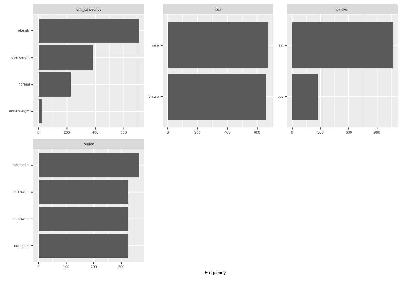
Dataset contains BMI values studied subjects which was a calculation of a body person’s weight (in kilograms) divided by the square of their height (in meters). We will categorize this this values into four classes according to the CDC recommendation:
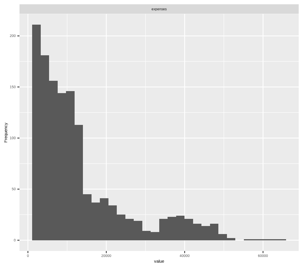
Then we will use plot_histogram() function of {DataExpler} package to see the distribution expenses data.
Code
mf |> dplyr::select(expenses) |>plot_histogram()
Code
moments::skewness(mf$expenses, na.rm =TRUE)
[1] 1.51418
High positive value indicates that the distribution is highly skewed at right-hand sight, which means that in some individual have high expenses (>20,000) in health insurance.
plot_bar() function from {DataExploer} package create frequency distribution of expenses, based on bmi, _catagories, sex, smoking and regions:
We will split the data into training and testing sets based on the bmi_categories, and sex variables. The training set will contain 70% of the data, and the testing set will contain the remaining 30%.
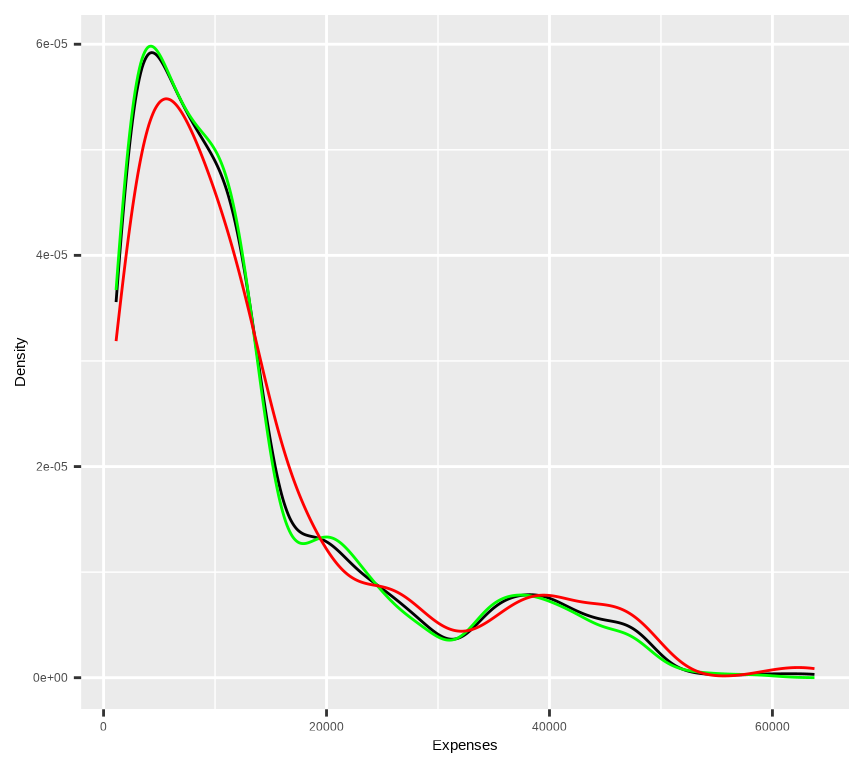
# Density plot all, train and test data ggplot()+geom_density(data = mf, aes(expenses))+geom_density(data = train, aes(expenses), color ="green")+geom_density(data = test, aes(expenses), color ="red") +xlab("Expenses") +ylab("Density")
Fit a Gamma Model in R
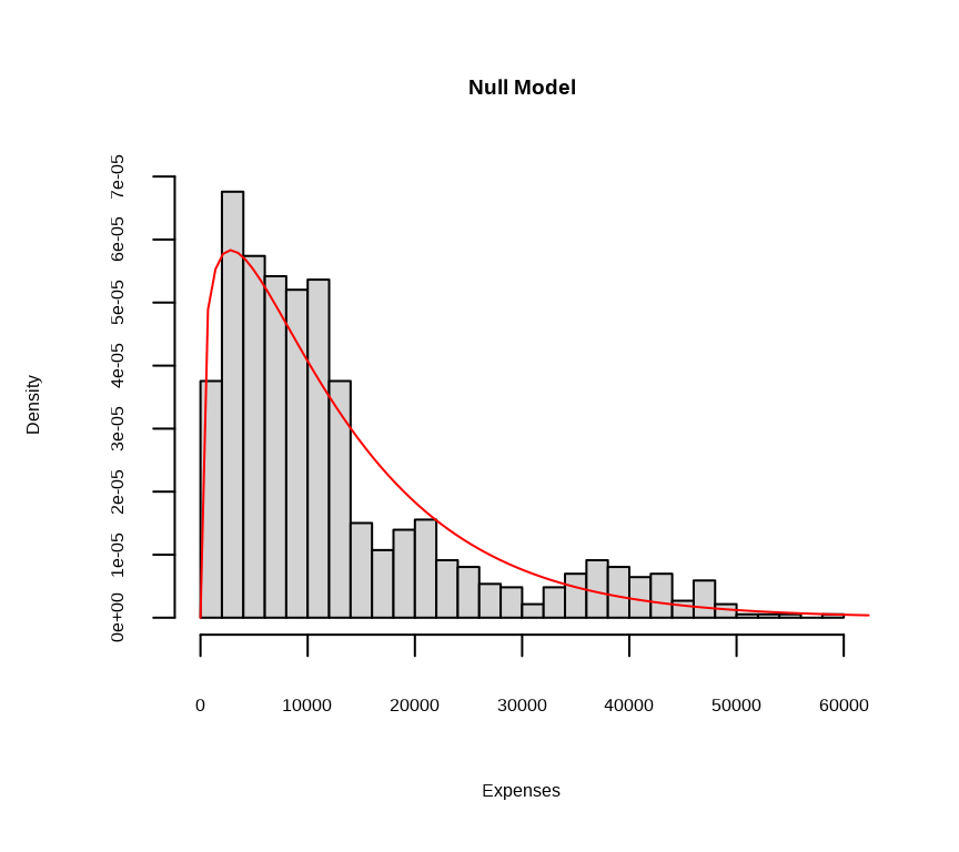
Only Intercept model
First we will fit Gamma model with intercept-only. l. This means modeling the data with no predictors. For gamma models, this would mean estimating the shape and scale parameters of the data. Notice we set link = "log". This is in response to errors and warnings that we received when using link = "identity" and link = "inverse" to fit more complicated models
Code
# Fit the ordinal logistic regression modelinter.gamma<-glm(expenses ~1, data =train, family =Gamma(link ="log"))summary(inter.gamma)
Call:
glm(formula = expenses ~ 1, family = Gamma(link = "log"), data = train)

Coefficients:
            Estimate Std. Error t value Pr(>|t|)
(Intercept)  9.46533    0.02974   318.3   <2e-16 ***
---
Signif. codes:  0 '***' 0.001 '**' 0.01 '*' 0.05 '.' 0.1 ' ' 1

(Dispersion parameter for Gamma family taken to be 0.8244218)

    Null deviance: 728.98  on 931  degrees of freedom
Residual deviance: 728.98  on 931  degrees of freedom
AIC: 19454

Number of Fisher Scoring iterations: 5
From above output, we notice the null and residual deviance are identical. The null deviance always reports deviance for the intercept-only model.
If we exponentiate the intercept we get the overall mean of expenses.
Code
exp(coef(inter.gamma))
(Intercept)
   12904.54
In the Gamma family, the dispersion parameter can be estimated from the deviance and the degrees of freedom in the summary output.
Code
# Extract deviance and residual degrees of freedom from the model summarydeviance_val <- inter.gamma$devianceresidual_df <- inter.gamma$df.residua# Calculate the dispersion parameterdispersion_parameter <- deviance_val / residual_dfdispersion_parameter
[1] 0.7830084
We can also extract the estimated shape and scale parameters as follows:
Now let’s use the estimated shape and scale parameters to draw the estimated gamma distribution on top of a histogram of the observed data.
Code
hist(train$expenses, breaks =40, freq =FALSE, xlab ="Expenses",main="Null Model")curve(dgamma(x, shape = inter.gamma_shape , scale = inter.gamma_scale ), from =0, to =70000, col ="red", add =TRUE, )
Full Model
Now, let’s fit a Gamma regression model. We’ll predict charges using age, sex, bmi_cra children, smoker, and region. We’ll use a log link function to ensure the predicted values are positive.
Code
# Fit the gamma modelfit.gamma<-glm(expenses~bmi_categories + sex + smoker + region + children + age, data= train,family =Gamma(link ="log"))
Model Summary
Code
summary(fit.gamma)
Call:
glm(formula = expenses ~ bmi_categories + sex + smoker + region +
    children + age, family = Gamma(link = "log"), data = train)

Coefficients:
                          Estimate Std. Error t value Pr(>|t|)
(Intercept)               7.506578   0.196173  38.265  < 2e-16 ***
bmi_categoriesnormal      0.273121   0.192829   1.416  0.15700
bmi_categoriesoverweight  0.295163   0.189897   1.554  0.12045
bmi_categoriesobesity     0.428294   0.188581   2.271  0.02337 *
sexmale                  -0.052456   0.045269  -1.159  0.24686
smokeryes                 1.502742   0.057614  26.083  < 2e-16 ***
regionnorthwest          -0.084428   0.065172  -1.295  0.19549
regionsoutheast          -0.192420   0.064621  -2.978  0.00298 **
regionsouthwest          -0.164759   0.065054  -2.533  0.01149 *
children                  0.090770   0.019304   4.702 2.97e-06 ***
age                       0.027960   0.001627  17.182  < 2e-16 ***
---
Signif. codes:  0 '***' 0.001 '**' 0.01 '*' 0.05 '.' 0.1 ' ' 1

(Dispersion parameter for Gamma family taken to be 0.4746951)

    Null deviance: 728.98  on 931  degrees of freedom
Residual deviance: 242.17  on 921  degrees of freedom
AIC: 18368

Number of Fisher Scoring iterations: 7
Check the Overall Model Fit
Code
anova(inter.gamma,fit.gamma)
Analysis of Deviance Table

Model 1: expenses ~ 1
Model 2: expenses ~ bmi_categories + sex + smoker + region + children +
    age
  Resid. Df Resid. Dev Df Deviance      F    Pr(>F)
1       931     728.98
2       921     242.17 10   486.81 102.55 < 2.2e-16 ***
---
Signif. codes:  0 '***' 0.001 '**' 0.01 '*' 0.05 '.' 0.1 ' ' 1
From the above output, you see that the chi-square is 242 and p = <0.0001. This means that you can reject the null hypothesis that the model without predictors is as good as the model with the predictors
Report Model Summary
Code
report::report(fit.gamma)
We fitted a general linear model (Gamma family with a log link) (estimated
using ML) to predict expenses with bmi_categories, sex, smoker, region,
children and age (formula: expenses ~ bmi_categories + sex + smoker + region +
children + age). The model's explanatory power is substantial (Nagelkerke's R2
= 0.75). The model's intercept, corresponding to bmi_categories = underweight,
sex = female, smoker = no, region = northeast, children = 0 and age = 0, is at
7.51 (95% CI [7.14, 7.91], t(921) = 38.27, p < .001). Within this model:

  - The effect of bmi categories [normal] is statistically non-significant and
positive (beta = 0.27, 95% CI [-0.13, 0.63], t(921) = 1.42, p = 0.157; Std.
beta = 0.27, 95% CI [-0.13, 0.63])
  - The effect of bmi categories [overweight] is statistically non-significant
and positive (beta = 0.30, 95% CI [-0.10, 0.65], t(921) = 1.55, p = 0.120; Std.
beta = 0.30, 95% CI [-0.10, 0.65])
  - The effect of bmi categories [obesity] is statistically significant and
positive (beta = 0.43, 95% CI [0.04, 0.78], t(921) = 2.27, p = 0.023; Std. beta
= 0.43, 95% CI [0.04, 0.78])
  - The effect of sex [male] is statistically non-significant and negative (beta
= -0.05, 95% CI [-0.14, 0.04], t(921) = -1.16, p = 0.247; Std. beta = -0.05,
95% CI [-0.14, 0.04])
  - The effect of smoker [yes] is statistically significant and positive (beta =
1.50, 95% CI [1.39, 1.62], t(921) = 26.08, p < .001; Std. beta = 1.50, 95% CI
[1.39, 1.62])
  - The effect of region [northwest] is statistically non-significant and
negative (beta = -0.08, 95% CI [-0.21, 0.04], t(921) = -1.30, p = 0.195; Std.
beta = -0.08, 95% CI [-0.21, 0.04])
  - The effect of region [southeast] is statistically significant and negative
(beta = -0.19, 95% CI [-0.32, -0.07], t(921) = -2.98, p = 0.003; Std. beta =
-0.19, 95% CI [-0.32, -0.07])
  - The effect of region [southwest] is statistically significant and negative
(beta = -0.16, 95% CI [-0.29, -0.04], t(921) = -2.53, p = 0.011; Std. beta =
-0.16, 95% CI [-0.29, -0.04])
  - The effect of children is statistically significant and positive (beta =
0.09, 95% CI [0.05, 0.13], t(921) = 4.70, p < .001; Std. beta = 0.11, 95% CI
[0.06, 0.15])
  - The effect of age is statistically significant and positive (beta = 0.03, 95%
CI [0.02, 0.03], t(921) = 17.18, p < .001; Std. beta = 0.39, 95% CI [0.35,
0.44])

Standardized parameters were obtained by fitting the model on a standardized
version of the dataset. 95% Confidence Intervals (CIs) and p-values were
computed using a Wald t-distribution approximation.
The tbl_regression() function from the gtsummary package takes a regression model object as input and produces a formatted table with Odd-ratio and confidence interval.
Code
tbl_regression(fit.gamma, exp =TRUE)
Characteristic
exp(Beta)
95% CI
p-value
bmi_categories
underweight
—
—
normal
1.31
0.88, 1.88
0.2
overweight
1.34
0.91, 1.91
0.12
obesity
1.53
1.04, 2.18
0.023
sex
female
—
—
male
0.95
0.87, 1.04
0.2
smoker
no
—
—
yes
4.49
4.01, 5.05
<0.001
region
northeast
—
—
northwest
0.92
0.81, 1.04
0.2
southeast
0.82
0.73, 0.94
0.003
southwest
0.85
0.75, 0.96
0.011
children
1.10
1.05, 1.14
<0.001
age
1.03
1.03, 1.03
<0.001
Abbreviation: CI = Confidence Interval
The tab_model() function of {sjPlot} package also creates HTML tables from regression models:
Code
tab_model(fit.gamma)
expenses
Predictors
Estimates
CI
p
(Intercept)
1819.98
1258.72 – 2734.20
<0.001
bmi categories [normal]
1.31
0.88 – 1.88
0.157
bmi categories
[overweight]
1.34
0.91 – 1.91
0.120
bmi categories [obesity]
1.53
1.04 – 2.18
0.023
sex [male]
0.95
0.87 – 1.04
0.247
smoker [yes]
4.49
4.01 – 5.05
<0.001
region [northwest]
0.92
0.81 – 1.04
0.195
region [southeast]
0.82
0.73 – 0.94
0.003
region [southwest]
0.85
0.75 – 0.96
0.011
children
1.10
1.05 – 1.14
<0.001
age
1.03
1.03 – 1.03
<0.001
Observations
932
R2 Nagelkerke
0.750
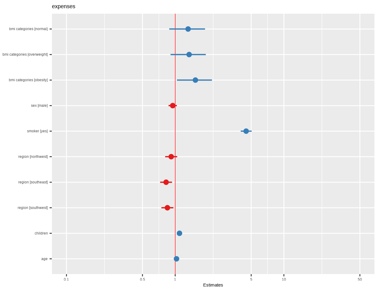
plot_model() function of {sjPlot} package creates plots the estimates from logistic model:
Code
plot_model(fit.gamma, vline.color ="red")
Shape and Scale of the Fitted Model
Code
# Calculate mean and variance of predicted valuespredicted_mu <-fitted(fit.gamma)mean_mu <-mean(predicted_mu)var_mu <-var(predicted_mu)# Estimate shape (k) and scale (theta)shape_estimate <- mean_mu^2/ var_muscale_estimate <- var_mu / mean_mucat("Estimated shape (k):", shape_estimate, "\n")
Now let’s use the estimated shape and scale parameters to draw the estimated gamma distribution on top of a histogram of the observed data.
Code
hist(train$expenses, breaks =40, freq =FALSE, xlab ="Expenses",main="Full Model")curve(dgamma(x, shape = shape_estimate, scale = scale_estimate ), from =0, to =70000, col ="red", add =TRUE, )
Model Performance
Code
performance::performance(fit.gamma)
# Indices of model performance

AIC       |      AICc |       BIC | Nagelkerke's R2 |     RMSE | Sigma
----------------------------------------------------------------------
18367.545 | 18367.884 | 18425.593 |           0.750 | 7746.727 | 0.689
Marginal Effect
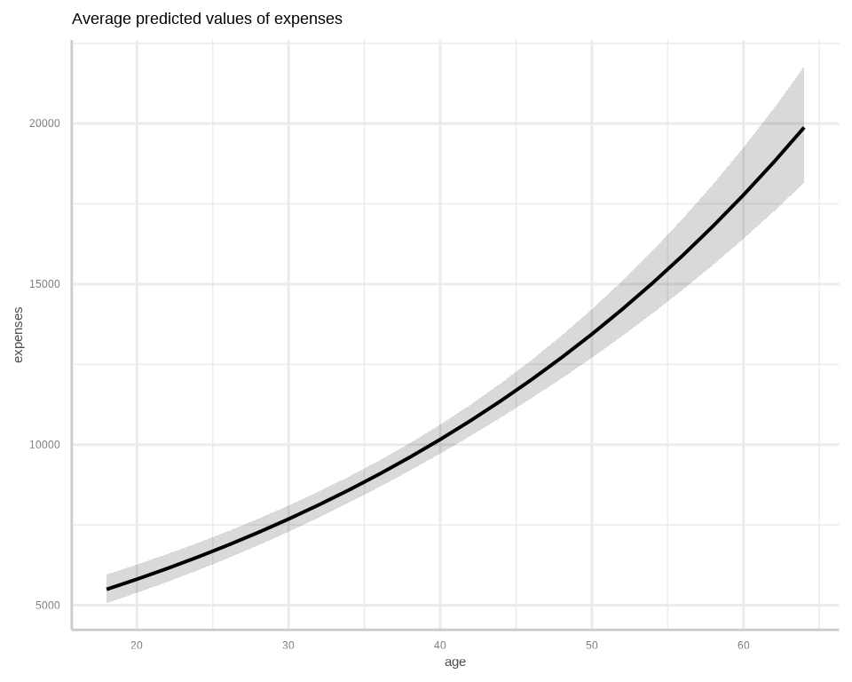
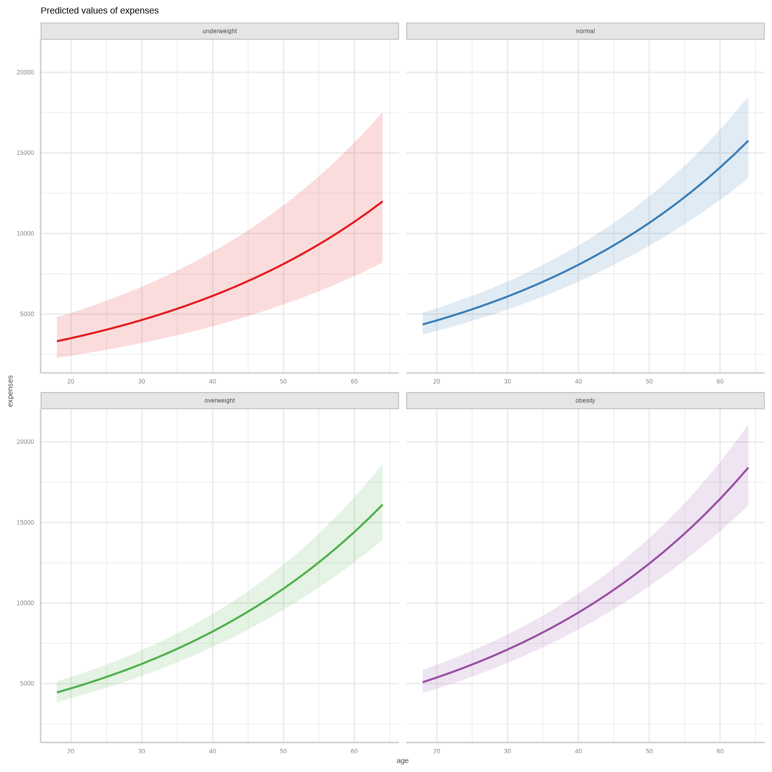
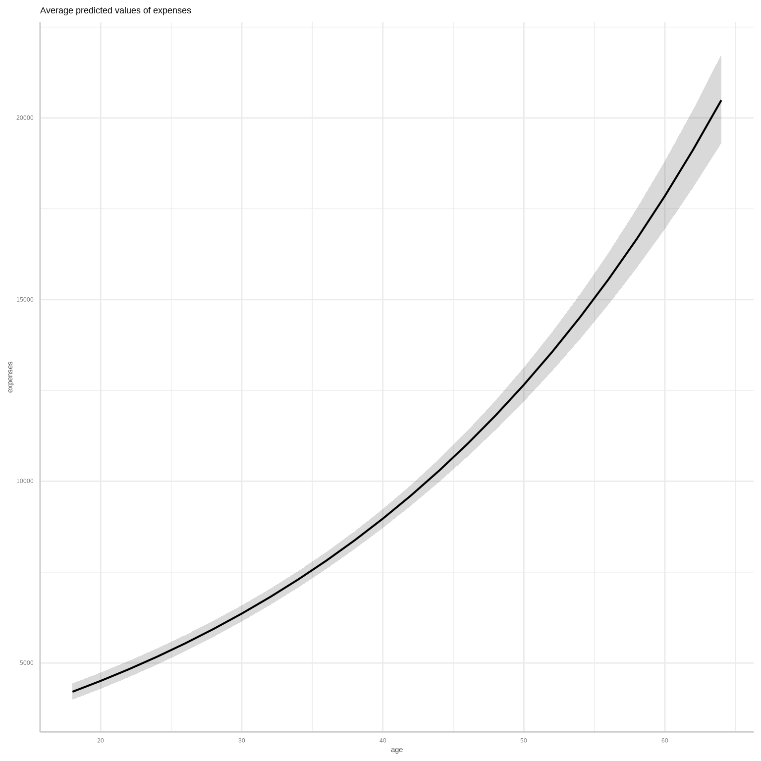
To calculate marginal effects and adjusted predictions, the predict_response() function of {ggeffects} package is used. This function can return three types of predictions, namely, conditional effects, marginal effects or marginal means, and average marginal effects or counterfactual predictions. You can set the type of prediction you want by using the margin argument.
We’ll use 5-fold cross-validation to evaluate the model’s predictive performance using the Mean Squared Error (MSE) as the metric.
Code
# Define MSE functionmse <-function(actual, predicted) {mean((actual - predicted)^2)}# Set up cross-validationset.seed(42)k_folds <-5folds <-sample(rep(1:k_folds, length.out =nrow(mf)))mse_values <-numeric(k_folds)for (i in1:k_folds) {# Split data into training and validation sets train_index <-which(folds != i) test_index <-which(folds == i) train_data <- mf[train_index, ] test_data <- mf[test_index, ]# Fit the Gamma model on training data cv_model <-glm(expenses ~ age + sex + bmi_categories + children + smoker + region, data = train_data, family =Gamma(link ="log"))# Predict on the validation set predictions <-predict(cv_model, newdata = test_data, type ="response")# Calculate MSE for the fold mse_values[i] <-mse(test_data$expenses, predictions)}# Average MSE across all foldsaverage_mse_cv <-mean(mse_values)cat("Average MSE from cross-validation:", average_mse_cv, "\n")
Average MSE from cross-validation: 63856032
Prediction at Test data
Code
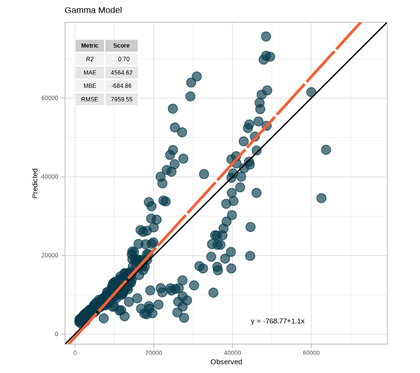
# Predict on the test settest$Pred.gamma <-predict(fit.gamma, newdata = test, type ="response")
test.metrica.plot <-scatter_plot(data = test,obs = expenses, pred = Pred.gamma,print_metrics =TRUE, metrics_list = my.metrics,position_metrics =c(x =10, y =75000)) +ggtitle("Gamma Model") +theme_light()test.metrica.plot
Log Linear model
It’s important to note that traditional linear modeling with a log transformation can be just as effective as gamma regression in some cases. To illustrate this, we’ll use the lm() function to fit a simple linear model with the total value log-transform. Oeef
Code
fit.lm<-glm(log(expenses)~bmi_categories + sex + smoker + region + children + age, data= train)summary(fit.lm)
Call:
glm(formula = log(expenses) ~ bmi_categories + sex + smoker +
    region + children + age, data = train)

Coefficients:
                          Estimate Std. Error t value Pr(>|t|)
(Intercept)               7.228502   0.128637  56.193  < 2e-16 ***
bmi_categoriesnormal      0.114645   0.126444   0.907 0.364809
bmi_categoriesoverweight  0.175631   0.124521   1.410 0.158743
bmi_categoriesobesity     0.300275   0.123658   2.428 0.015361 *
sexmale                  -0.073391   0.029684  -2.472 0.013602 *
smokeryes                 1.555938   0.037779  41.185  < 2e-16 ***
regionnorthwest          -0.092564   0.042735  -2.166 0.030569 *
regionsoutheast          -0.185469   0.042374  -4.377 1.34e-05 ***
regionsouthwest          -0.144643   0.042658  -3.391 0.000727 ***
children                  0.109304   0.012658   8.635  < 2e-16 ***
age                       0.034409   0.001067  32.247  < 2e-16 ***
---
Signif. codes:  0 '***' 0.001 '**' 0.01 '*' 0.05 '.' 0.1 ' ' 1

(Dispersion parameter for gaussian family taken to be 0.2041099)

    Null deviance: 780.74  on 931  degrees of freedom
Residual deviance: 187.99  on 921  degrees of freedom
AIC: 1176.8

Number of Fisher Scoring iterations: 2
Coefficients in linear model slightly different than Gamma model, but overall interpretation is almost identical:
In this tutorial, we covered the essentials of Gamma regression in R, focusing on a manual approach and the implementation using R’s glm() function. We discussed when to use Gamma regression, particularly for non-negative, skewed data with increasing variance, which is common in finance, healthcare, environmental science, and engineering. Implementing Gamma regression from scratch helped us understand the model’s mechanics, including the log-likelihood function and coefficient estimation. We then utilized R’s glm() function to fit a Gamma regression model more efficiently, emphasizing its simplicity in estimating parameters and interpreting output metrics like coefficients, standard errors, and goodness-of-fit measures. Gamma regression is vital for analyzing non-negative continuous data with a right-skewed distribution. With the knowledge gained in this tutorial, you can effectively apply Gamma regression to various real-world datasets, providing more accurate insights and predictions in fields such as claims costs, waiting times, and biological measurements.