Code
# Packages List
packages <- c(
  "tidyverse",   # Includes readr, dplyr, ggplot2, etc.
  'patchwork', # for visualization
  'minpack.lm', # for damped exponential model
  'nlstools' # for bootstrapping
)![]()

Exponential models are a type of non-linear regression model that describes exponential growth or decay in a variable. Exponential models are widely used in various fields such as biology, finance, physics, and engineering to describe phenomena that exhibit exponential behavior. In this tutorial, we will explore exponential models, their applications, and how to fit exponential models in R.
Exponential Growth: Exponential growth models describe phenomena where a quantity increases at a rate proportional to its current value. Mathematically, exponential growth is represented by the equation \(y = a \cdot e^{bx}\), where \(a\) is the initial value and \(b\) is the growth rate.
Exponential Decay: Exponential decay models describe phenomena where a quantity decreases at a rate proportional to its current value. Mathematically, exponential decay is represented by the equation \(y = a \cdot e^{-bx}\), where \(a\) is the initial value and \(b\) is the decay rate.
Applications: Exponential models are used to describe a wide range of natural phenomena, such as population growth, radioactive decay, compound interest, and more.
Exponential models can be fitted using non-linear regression techniques such as the least squares method or the Gauss-Newton algorithm. These methods estimate the parameters of the exponential model by minimizing the sum of squared residuals between the observed and predicted values.
# Packages List
packages <- c(
"tidyverse", # Includes readr, dplyr, ggplot2, etc.
'patchwork', # for visualization
'minpack.lm', # for damped exponential model
'nlstools' # for bootstrapping
)#| warning: false
#| error: false
# Install missing packages
new_packages <- packages[!(packages %in% installed.packages()[,"Package"])]
if(length(new_packages)) install.packages(new_packages)
# Verify installation
cat("Installed packages:\n")
print(sapply(packages, requireNamespace, quietly = TRUE))# Load packages with suppressed messages
invisible(lapply(packages, function(pkg) {
suppressPackageStartupMessages(library(pkg, character.only = TRUE))
}))# Check loaded packages
cat("Successfully loaded packages:\n")Successfully loaded packages:print(search()[grepl("package:", search())]) [1] "package:nlstools" "package:minpack.lm" "package:patchwork"
[4] "package:lubridate" "package:forcats" "package:stringr"
[7] "package:dplyr" "package:purrr" "package:readr"
[10] "package:tidyr" "package:tibble" "package:ggplot2"
[13] "package:tidyverse" "package:stats" "package:graphics"
[16] "package:grDevices" "package:utils" "package:datasets"
[19] "package:methods" "package:base" Exponential models are mathematical functions that describe exponential growth or decay. These models are used in various fields such as finance, biology, physics, and economics. Below are the different types of exponential models:
\[ y = a e^{bx} \] where: - \(y\) is the output, - \(a\)) is the initial value (when \(x = 0\)), - \(b\) is the growth rate (\(b > 0\)), - \(e\) is Euler’s number (\(\approx 2.718\)), - \(x\) is the independent variable (often time).
Exponential Decay Model
Formula:
\[ y = a e^{- bx} \]
where \(b > 0\), leading to a decreasing function.
Characteristics:
Below is an example of how to fit a Exponential Growth and Decay Models in R using nonlinear least squares:
You’ll need the nls() (nonlinear least squares) function for fitting nonlinear models and ggplot2 for visualization.
# Generate synthetic data
set.seed(123)  # For reproducibility
x <- seq(0, 10, length.out = 100)

# Exponential Growth Data (y = a * exp(b * x))
y_growth <- 2 * exp(0.3 * x) + rnorm(100, 0, 2)  # Adding noise
growth_data <- data.frame(x, y_growth)

# Exponential Decay Data (y = a * exp(-b * x))
y_decay <- 10 * exp(-0.4 * x) + rnorm(100, 0, 1)  # Adding noise
decay_data <- data.frame(x, y_decay)

# ---- Fit Exponential Growth Model ----
growth_model <- nls(y_growth ~ a * exp(b * x), data = growth_data,
                    start = list(a = 1, b = 0.1))
growth_data$growth_pred <- predict(growth_model)

# ---- Fit Exponential Decay Model ----
decay_model <- nls(y_decay ~ a * exp(-b * x), data = decay_data,
                   start = list(a = 10, b = 0.2))
decay_data$decay_pred <- predict(decay_model)# ---- Plot Exponential Growth ----
p1 <- ggplot(growth_data, aes(x)) +
geom_point(aes(y = y_growth), color = "blue", alpha = 0.5) + # Actual data points
geom_line(aes(y = growth_pred), color = "blue", size = 1) + # Fitted curve
ggtitle("Exponential Growth Fit") +
theme_minimal()Warning: Using `size` aesthetic for lines was deprecated in ggplot2 3.4.0.
ℹ Please use `linewidth` instead.# ---- Plot Exponential Decay ----
p2 <- ggplot(decay_data, aes(x)) +
geom_point(aes(y = y_decay), color = "red", alpha = 0.5) + # Actual data points
geom_line(aes(y = decay_pred), color = "red", size = 1) + # Fitted curve
ggtitle("Exponential Decay Fit") +
theme_minimal()
# Display both plots
library(gridExtra)
Attaching package: 'gridExtra'The following object is masked from 'package:dplyr':
combinegrid.arrange(p1, p2, ncol = 2)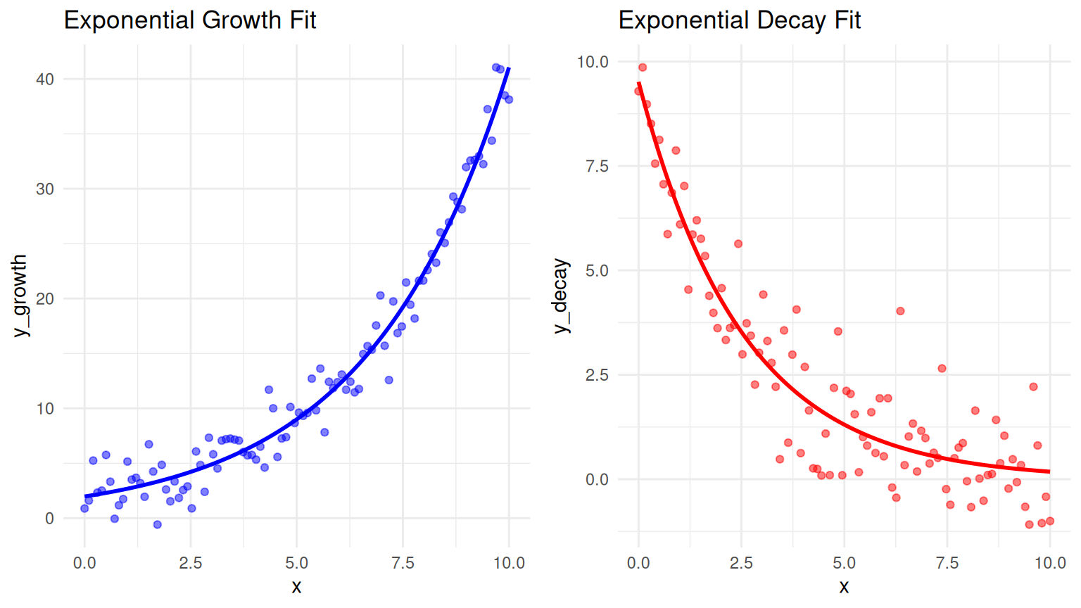
A double exponential growth model describes a process where the quantity grows at an accelerating rate, meaning the growth rate itself is growing exponentially. This model is characterized by a positive second growth rate. It is often used in contexts where growth accelerates over time, such as in certain financial markets, technological advancements, or biological phenomena.
The general form of a double exponential growth model is:
\[ y = a \cdot e^{b \cdot e^{cx}} \]
where: - \(y\) is the dependent variable. - \(x\) is the independent variable. - \(a\) is the initial value (the value of \(y\) when \(x = 0\)). - \(b\) and \(c\) are positive growth rates. - \(e\) is the base of the natural logarithm (approximately equal to 2.71828).
Below is an example of how to fit a double exponential growth model in R using nonlinear least squares:
# Generate example data
set.seed(123)
x <- seq(0, 10, by = 0.2)
a <- 2
b <- 0.5
c <- 0.3
y <- a * exp(b * exp(c * x)) + rnorm(length(x), sd = 10)

# Define the double exponential growth model function
double_exp_model <- function(params, x) {
  a <- params[1]
  b <- params[2]
  c <- params[3]
  a * exp(b * exp(c * x))
}

# Define the residual function for nonlinear least squares
residuals <- function(params, x, y) {
  y - double_exp_model(params, x)
}

# Initial parameter guesses
init_params <- c(a = 1, b = 0.1, c = 0.1)

# Fit the model using nonlinear least squares
fit <- nls.lm(par = init_params, fn = residuals, x = x, y = y)
Warning in nls.lm(par = init_params, fn = residuals, x = x, y = y): lmdif: info = -1. Number of iterations has reached `maxiter' == 50.# Extract fitted parameters
fitted_params <- fit$par
print(fitted_params) a b c
2.0739010 0.4922369 0.3012036 # Generate fitted values
y_fitted <- double_exp_model(fitted_params, x)
# Plot the data and fitted model
plot_data <- data.frame(x = x, y = y, y_fitted = y_fitted)
ggplot(plot_data, aes(x = x)) +
geom_point(aes(y = y), color = 'blue', size = 1) +
geom_line(aes(y = y_fitted), color = 'red', size = 1) +
ggtitle('Double Exponential Growth Model Fit') +
xlab('Independent Variable (x)') +
ylab('Dependent Variable (y)') +
theme_minimal()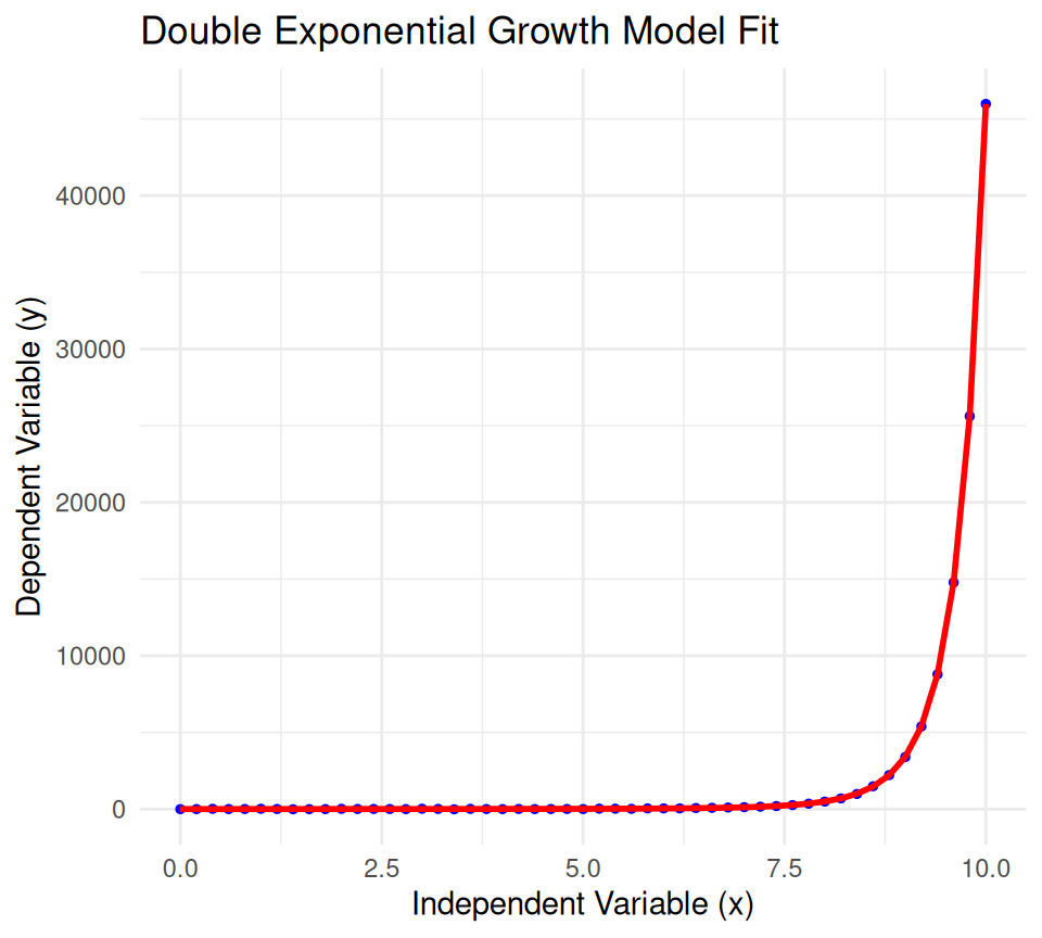
A damped exponential model describes a process where the amplitude of the oscillations decreases over time. This model is often used in physics and engineering to describe systems that exhibit damped harmonic motion, such as a mass-spring-damper system.
The general form of a damped exponential model is:
\[ y(t) = A \cdot e^{-\lambda t} \cdot \cos(\omega t + \phi) \]
where: - \(y(t)\) is the dependent variable at time \(t\). - \(A\) is the initial amplitude. - \(\lambda\) is the damping coefficient. - \(\omega\) is the angular frequency. - \(\phi\) is the phase shift. - \(e\) is the base of the natural logarithm (approximately equal to 2.71828).
Applications - Mechanical systems with damping (e.g., mass-spring-damper systems) - Electrical circuits with resistance (e.g., RLC circuits) - Biological systems (e.g., neuron firing patterns)
Below is an example of how to fit a damped exponential model in R using nonlinear least squares:
# Generate example data
set.seed(123)
t <- seq(0, 10, by = 0.1)
A <- 5
lambda <- 0.3
omega <- 2 * pi * 0.5
phi <- pi / 4
y <- A * exp(-lambda * t) * cos(omega * t + phi) + rnorm(length(t), sd = 0.5)
# Define the damped exponential model function
damped_exp_model <- function(params, t) {
A <- params[1]
lambda <- params[2]
omega <- params[3]
phi <- params[4]
A * exp(-lambda * t) * cos(omega * t + phi)
}
# Define the residual function for nonlinear least squares
residuals <- function(params, t, y) {
y - damped_exp_model(params, t)
}
# Initial parameter guesses
init_params <- c(A = 5, lambda = 0.3, omega = 2 * pi * 0.5, phi = pi / 4)
# Fit the model using nonlinear least squares
fit <- nls.lm(par = init_params, fn = residuals, t = t, y = y)
# Extract fitted parameters
fitted_params <- fit$par
print(fitted_params) A lambda omega phi
4.9541405 0.3033703 3.1848578 0.7603952 # Generate fitted values
y_fitted <- damped_exp_model(fitted_params, t)
# Plot the data and fitted model
plot_data <- data.frame(t = t, y = y, y_fitted = y_fitted)
ggplot(plot_data, aes(x = t)) +
geom_point(aes(y = y), color = 'blue', size = 1) +
geom_line(aes(y = y_fitted), color = 'red', size = 1) +
ggtitle('Damped Exponential Model Fit') +
xlab('Time (t)') +
ylab('Amplitude (y)') +
theme_minimal()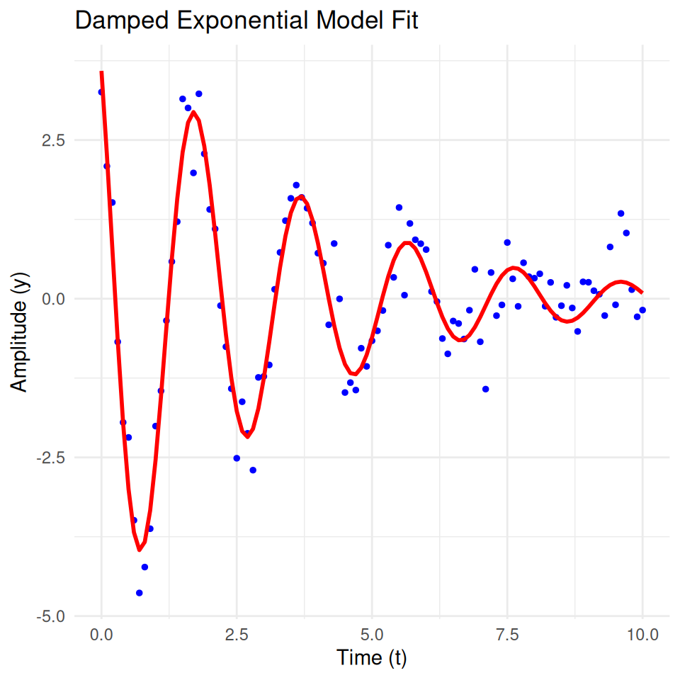
In this section, we will fit an exponential model to real-world data using R. We will use a dataset, which contains information about Arsenic (As) content in rice vaegeative parts (STAs) and Tansfer Factor (ratio of As in grain and straw). We will fit an exponential growth model to the relationship between STAs and TF to explore TF changes as As uptake increases by rice.
# Load data
mf<-readr::read_csv("https://github.com/zia207/r-colab/raw/main/Data/Regression_analysis/tf_data.csv") |>
  glimpse()
Rows: 260
Columns: 3
$ STAs <dbl> 0.9, 1.0, 1.6, 1.6, 1.6, 1.8, 1.9, 2.2, 2.3, 2.4, 2.5, 2.5, 2…
$ TF <dbl> 0.13888889, 0.09400000, 0.06750000, 0.09187500, 0.06062500, 0…
$ Rice_Var <chr> "Purbachi", "Purbachi", "Ratna", "Purbachi", "Purbachi", "Pur…ggplot(mf, aes(x = STAs, y = TF)) +
geom_point(alpha = 0.6, color = "blue") +
labs(title = "TF vs. Straw As ", x = "As (ppm)", y = "TF") +
theme_minimal()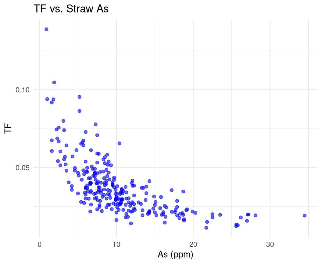
First we will performed Log-Transformation of the data to linearize the relationship for fitting:
# Add log(TF) column (avoid log(0) issues)
mf <- mf  |>
  mutate(logTF = log(TF))  # Already provided in your CSV, but we recalculate here

# Plot transformed data
ggplot(mf, aes(x = STAs, y = logTF)) +
  geom_point(alpha = 0.6, color = "red") +
  labs(title = "log(TF) vs. STAs  (Linearized)", x = "As (ppm)", y = "log(TF)") +
  theme_minimal()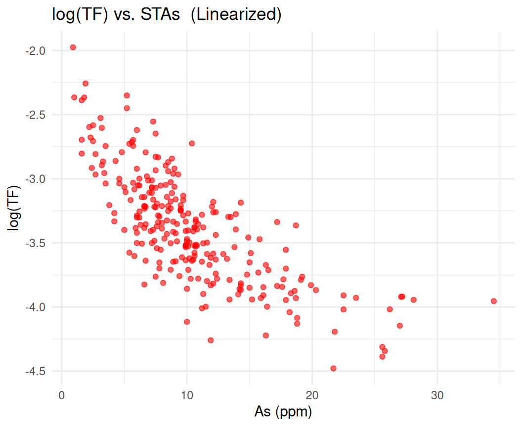
Now, we fit an exponential decay model to the log-transformed data using nonlinear least squares:
# Fit model: log(TF) = β₀ + β₁ * stas
model.exp <- lm(log(TF) ~ STAs, data = mf)

# Summary of results
summary(model.exp)
Call:
lm(formula = log(TF) ~ STAs, data = mf)

Residuals:
     Min       1Q   Median       3Q      Max
-0.78385 -0.19435 -0.01188  0.18099  0.85474

Coefficients:
             Estimate Std. Error t value Pr(>|t|)
(Intercept) -2.774480   0.037201  -74.58   <2e-16 ***
STAs        -0.058992   0.003173  -18.59   <2e-16 ***
---
Signif. codes:  0 '***' 0.001 '**' 0.01 '*' 0.05 '.' 0.1 ' ' 1

Residual standard error: 0.2835 on 258 degrees of freedom
Multiple R-squared:  0.5726,    Adjusted R-squared:  0.5709
F-statistic: 345.6 on 1 and 258 DF,  p-value: < 2.2e-16
Inntercept (β₀): Estimated log(A) in the exponential model TF = A * e^(β₁ * stas).
Slope (β₁): Decay rate (since TF decreases as stas increases).
Use exp(coef(model)[1]) to recover A.
# Extract model parameters
A <- exp(coef(model.exp)[1])  # Initial value (when stas = 0)
beta <- coef(model.exp)[2]    # Decay rate

cat("Exponential model: TF =", round(A, 4), "* e^(", round(beta, 4), "* STAs)")
Exponential model: TF = 0.0624 * e^( -0.059 * STAs)# Add predictions to the data
mf$predicted <- exp(predict(model.exp))
# Plot raw data and fitted curve
ggplot(mf, aes(x = STAs, y = TF)) +
geom_point(alpha = 0.6, color = "blue") +
geom_line(aes(y = predicted), color = "red", linewidth = 1) +
labs(title = "Exponential Model Fit", x = "As (ppm)", y = "TF") +
theme_minimal()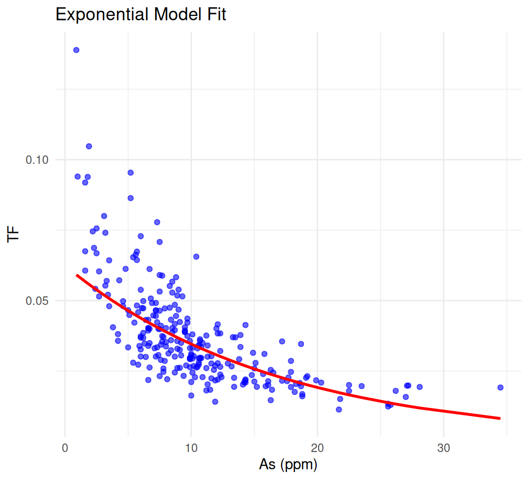
We can also use nls() function to fit an exponential model to the data:
# Define the exponential model function
exp_model <- function(params, x) {
  a <- params[1]
  b <- params[2]
  a * exp(b * x)
}

# Define the residual function for nonlinear least squares
residuals <- function(params, x, y) {
  y - exp_model(params, x)
}

# Initial parameter guesses
init_params <- c(a = 0.1, b = -0.1)

# Fit the model using nonlinear least squares
fit <- nls.lm(par = init_params, fn = residuals, x = mf$STAs, y = mf$TF)

# Extract fitted parameters
fitted_params <- fit$par
print(fitted_params)
a b
0.08323492 -0.08845286 # Generate fitted values
y_fitted <- exp_model(fitted_params, mf$STAs)
# Plot the data and fitted model
plot_data <- data.frame(STAs = mf$STAs, TF = mf$TF, y_fitted = y_fitted)
ggplot(plot_data, aes(x = STAs)) +
geom_point(aes(y = TF), color = 'blue', size = 1) +
geom_line(aes(y = y_fitted), color = 'red', size = 1) +
ggtitle('Exponential Model Fit') +
xlab('STAs') +
ylab('TF') +
theme_minimal()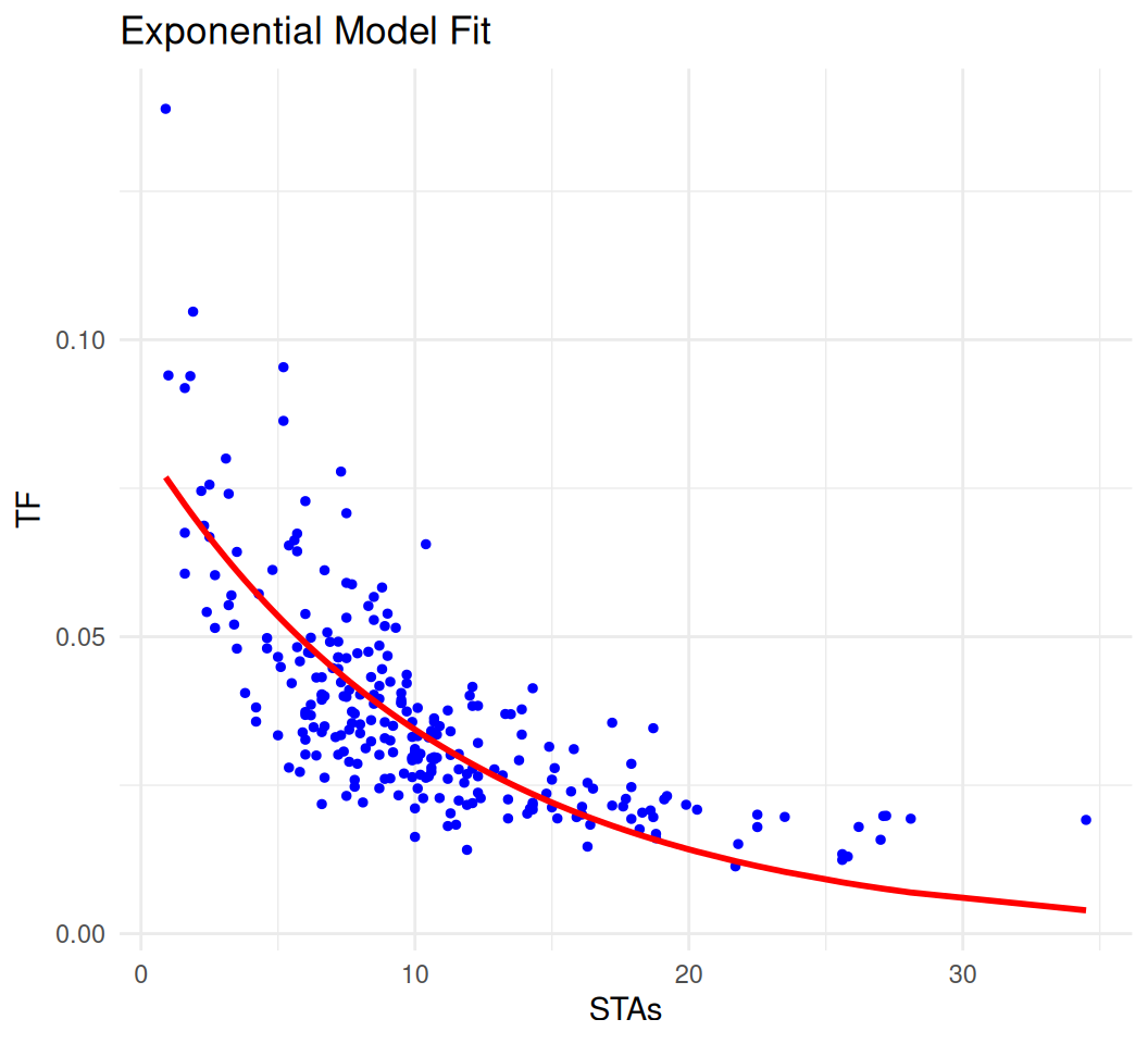
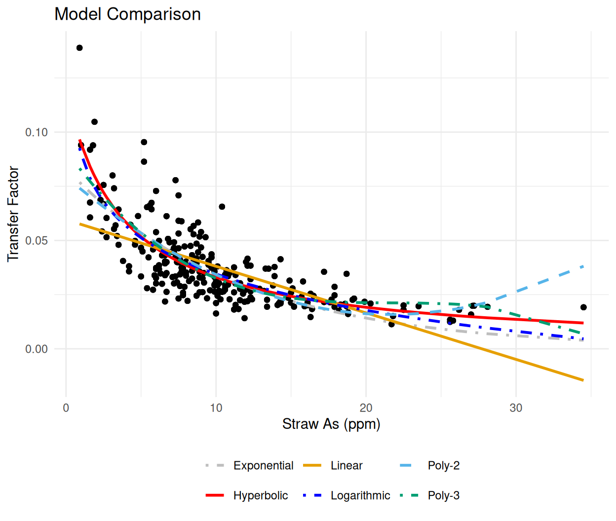
Now we can fit exponential model to the data and compare it with other models like linear, polynomial, logarithmic, and hyperbolic models to determine the best fitting model based on the R-squared value.
# Linear model
linear_model <- lm(TF ~ STAs, data = mf)
summary(linear_model)
Call:
lm(formula = TF ~ STAs, data = mf)

Residuals:
      Min        1Q    Median        3Q       Max
-0.023552 -0.008652 -0.002140  0.005127  0.081270

Coefficients:
             Estimate Std. Error t value Pr(>|t|)
(Intercept)  0.059553   0.001747   34.09   <2e-16 ***
STAs        -0.002149   0.000149  -14.42   <2e-16 ***
---
Signif. codes:  0 '***' 0.001 '**' 0.01 '*' 0.05 '.' 0.1 ' ' 1

Residual standard error: 0.01331 on 258 degrees of freedom
Multiple R-squared:  0.4464,    Adjusted R-squared:  0.4442
F-statistic: 208 on 1 and 258 DF, p-value: < 2.2e-16# Polynomial model (degree 2)
poly2_model <- lm(TF ~ poly(STAs, 2), data = mf)
summary(poly2_model)
Call:
lm(formula = TF ~ poly(STAs, 2), data = mf)

Residuals:
      Min        1Q    Median        3Q       Max
-0.024706 -0.006661 -0.001025  0.004815  0.064736

Coefficients:
                 Estimate Std. Error t value Pr(>|t|)
(Intercept)     0.0373524  0.0007182  52.010   <2e-16 ***
poly(STAs, 2)1 -0.1919900  0.0115802 -16.579   <2e-16 ***
poly(STAs, 2)2  0.1060970  0.0115802   9.162   <2e-16 ***
---
Signif. codes:  0 '***' 0.001 '**' 0.01 '*' 0.05 '.' 0.1 ' ' 1

Residual standard error: 0.01158 on 257 degrees of freedom
Multiple R-squared:  0.5827,    Adjusted R-squared:  0.5794
F-statistic: 179.4 on 2 and 257 DF, p-value: < 2.2e-16# Polynomial model (degree 3)
poly3_model <- lm(TF ~ poly(STAs, 3), data = mf)
summary(poly3_model)
Call:
lm(formula = TF ~ poly(STAs, 3), data = mf)

Residuals:
      Min        1Q    Median        3Q       Max
-0.023413 -0.006333 -0.001354  0.005036  0.055622

Coefficients:
                 Estimate Std. Error t value Pr(>|t|)
(Intercept)     0.0373524  0.0006926  53.927  < 2e-16 ***
poly(STAs, 3)1 -0.1919900  0.0111686 -17.190  < 2e-16 ***
poly(STAs, 3)2  0.1060970  0.0111686   9.500  < 2e-16 ***
poly(STAs, 3)3 -0.0503123  0.0111686  -4.505 1.01e-05 ***
---
Signif. codes:  0 '***' 0.001 '**' 0.01 '*' 0.05 '.' 0.1 ' ' 1

Residual standard error: 0.01117 on 256 degrees of freedom
Multiple R-squared:  0.6133,    Adjusted R-squared:  0.6088
F-statistic: 135.3 on 3 and 256 DF, p-value: < 2.2e-16# Exponential model
exp_model <- nls(TF ~ a * exp(b * STAs), data = mf, start = list(a = 0.1, b = -0.1))
summary(exp_model)
Formula: TF ~ a * exp(b * STAs)

Parameters:
   Estimate Std. Error t value Pr(>|t|)
a  0.083235   0.003211   25.93   <2e-16 ***
b -0.088453   0.004960  -17.83   <2e-16 ***
---
Signif. codes:  0 '***' 0.001 '**' 0.01 '*' 0.05 '.' 0.1 ' ' 1

Residual standard error: 0.01158 on 258 degrees of freedom

Number of iterations to convergence: 6
Achieved convergence tolerance: 3.842e-06
Logarithmic models are used when the rate of change in the data decreases over time or space. The general form of a logarithmic model is:
\[ y = a + b \cdot \ln(x) \]
where: - \(y\) is the dependent variable. - \(a\) and \(b\) are parameters that determine the shape of the curve. - \(\ln(x)\) is the natural logarithm of the independent variable \(x\).
# Logarithmic model
log_model <- lm(TF ~ log(STAs), data = mf)
summary(log_model)
Call:
lm(formula = TF ~ log(STAs), data = mf)

Residuals:
      Min        1Q    Median        3Q       Max
-0.022725 -0.006195 -0.001335  0.004821  0.046222

Coefficients:
             Estimate Std. Error t value Pr(>|t|)
(Intercept)  0.090122   0.002608   34.55   <2e-16 ***
log(STAs)   -0.024153   0.001153  -20.95   <2e-16 ***
---
Signif. codes:  0 '***' 0.001 '**' 0.01 '*' 0.05 '.' 0.1 ' ' 1

Residual standard error: 0.01089 on 258 degrees of freedom
Multiple R-squared:  0.6297,    Adjusted R-squared:  0.6282
F-statistic: 438.7 on 1 and 258 DF, p-value: < 2.2e-16A hyperbolic model is a type of mathematical model used to describe relationships that follow a hyperbolic distribution. In its simplest form, a hyperbolic model can be represented as:
\[ y = \frac{a}{b + x} \]
where: - \(y\) is the dependent variable. - \(a\) and \(b\) are parameters that determine the shape of the curve. - \(x\) is the independent variable.
# Hyperbolic model
hyperbolic_model <- nls(TF ~ a / (b + STAs), data = mf, start = list(a = 1, b = 1))
summary(hyperbolic_model)
Formula: TF ~ a/(b + STAs)

Parameters:
  Estimate Std. Error t value Pr(>|t|)
a  0.45618    0.02088  21.846   <2e-16 ***
b  3.82145    0.38951   9.811   <2e-16 ***
---
Signif. codes:  0 '***' 0.001 '**' 0.01 '*' 0.05 '.' 0.1 ' ' 1

Residual standard error: 0.01078 on 258 degrees of freedom

Number of iterations to convergence: 7
Achieved convergence tolerance: 8.432e-06metrics <- tibble(
Model = c("Linear", "Poly-2", "Poly-3", "Exponential", "Logarithmic", "Hyperbolic"),
RSE = c(summary(linear_model)$sigma,
summary(poly2_model)$sigma,
summary(poly3_model)$sigma,
summary(exp_model)$sigma,
summary(log_model)$sigma,
summary(hyperbolic_model)$sigma),
AIC = c(AIC(linear_model),
AIC(poly2_model),
AIC(poly3_model),
AIC(exp_model),
AIC(log_model),
AIC(hyperbolic_model)),
BIC = c(BIC(linear_model),
BIC(poly2_model),
BIC(poly3_model),
BIC(exp_model),
BIC(log_model),
BIC(hyperbolic_model)),
R2 = c(summary(linear_model)$r.squared,
summary(poly2_model)$r.squared,
summary(poly3_model)$r.squared,
1 - sum(resid(exp_model)^2) / sum((mf$TF - mean(mf$TF))^2), # Adjusted R-squared for nls
summary(log_model)$r.squared,
1- sum(resid(hyperbolic_model)^2) / sum((mf$TF - mean(mf$TF))^2)) # Adjusted R-squared for nls
)
metrics# A tibble: 6 × 5
Model RSE AIC BIC R2
<chr> <dbl> <dbl> <dbl> <dbl>
1 Linear 0.0133 -1504. -1493. 0.446
2 Poly-2 0.0116 -1576. -1561. 0.583
3 Poly-3 0.0112 -1593. -1576. 0.613
4 Exponential 0.0116 -1576. -1566. 0.581
5 Logarithmic 0.0109 -1609. -1598. 0.630
6 Hyperbolic 0.0108 -1614. -1603. 0.637best_model <- names(which.max(metrics$R2))
cat("Best model is:", best_model, "with R-squared value:", max(metrics$R2), "\n")Best model is: with R-squared value: 0.6371639 # Add predictions
mf<- mf %>%
mutate(
linear_pred = predict(linear_model),
poly2_pred = predict(poly2_model),
poly3_pred = predict(poly3_model),
exp_pred = predict(exp_model),
log_pred = predict(log_model),
hyper_pred = predict(hyperbolic_model)
)
# Reshape predictions into long format for legend
mf_long <- mf %>%
pivot_longer(
cols = c("linear_pred", "poly2_pred", "poly3_pred", "exp_pred", "log_pred", "hyper_pred"),
names_to = "Model",
values_to = "Prediction"
) %>%
mutate(
Model = case_when(
Model == "linear_pred" ~ "Linear",
Model == "poly2_pred" ~ "Poly-2",
Model == "poly3_pred" ~ "Poly-3",
Model == "exp_pred" ~ "Exponential",
Model == "log_pred" ~ "Logarithmic",
Model == "hyper_pred" ~ "Hyperbolic"
)
)
# Define colors and linetypes
model_colors <- c(
"Linear" = "#E69F00",
"Poly-2" = "#56B4E9",
"Poly-3" = "#009E73",
"Exponential" = "gray",
"Logarithmic" = "blue",
"Hyperbolic" = "red"
)
model_linetypes <- c(
"Linear" = "solid",
"Poly-2" = "dashed",
"Poly-3" = "dotdash",
"Exponential" = "dotdash",
"Logarithmic" = "dotdash",
"Hyperbolic" = "solid"
)
ggplot(mf_long, aes(x = STAs, y = TF)) +
geom_point(alpha = 0.6, color = "black") +
geom_line(
aes(y = Prediction, color = Model, linetype = Model),
linewidth = 1
) +
scale_color_manual(values = model_colors) +
scale_linetype_manual(values = model_linetypes) +
labs(
title = "Model Comparison",
x = "Straw As (ppm)",
y = "Transfer Factor"
) +
theme_minimal() +
theme(
legend.position = "bottom",
legend.title = element_blank(), # Remove legend title
legend.spacing.x = unit(0.5, "cm") # Add spacing between legend items
) +
guides(
color = guide_legend(nrow = 2), # Split color legend into 2 lines
linetype = guide_legend(nrow = 2) # Split linetype legend into 2 lines
)
In this R tutorial, we explored various types of exponential models and demonstrated how to fit them using R. Exponential models are powerful tools for describing processes that exhibit growth or decay at rates proportional to their current values. Here is a summary of what we covered:
For each type of model, we discussed the mathematical equations and provided R code to generate example data, fit the models using nonlinear least squares, and visualize the results using ggplot2. By understanding and applying these models, you can accurately capture and predict the behavior of various real-world phenomena that exhibit exponential growth or decay.
By mastering these techniques, you can leverage exponential models to gain insights and make predictions in diverse applications, ranging from biology and physics to finance and engineering.
Here are some books and online resources that provide comprehensive information about exponential models, including their applications, fitting techniques, and theoretical foundations:
nls function in R is used for fitting nonlinear models, including exponential models. The R documentation provides detailed information on how to use this function.